Advanced Filter with Criteria Range in Excel (18 Applications)

Method 1 – Using the Advanced Filter Criteria Range for Number and Dates

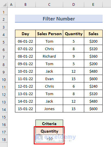
Column B to Column E in the sample dataset represents sales data. We will use the Advanced Filter Criteria Range for filtering numbers and date, extracting all data where the sales quantity is greater than 10.

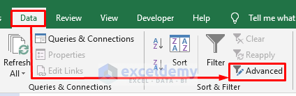
• In the Data tab, select the Advanced command from the Sort & Filter option. A dialogue box named Advanced Filter will appear.

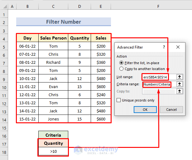
• Select the entire table (B4:E14) for the List range.
• Select cell (C17:C18) as Criteria range.
• Press OK.

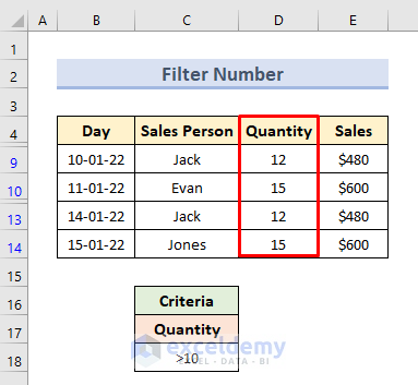
• Here’s the result.

Note:
1. Select the criteria with two rows at least.

2. We will use headers for the related columns where filtering criteria will be applied.

Method 2 – Filter Text Values with Advanced Filter Criteria

Case 2.1 – For Exact Text Match

We have the following dataset of sales along with a new column City. We will extract only the data for the city NEW YORK

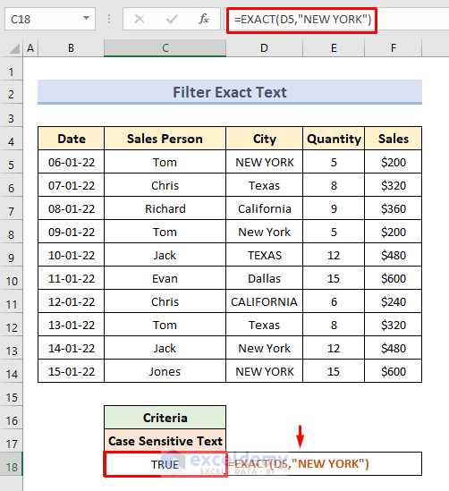
• Select cell C18.
• Insert the following formula:

• Press Enter.

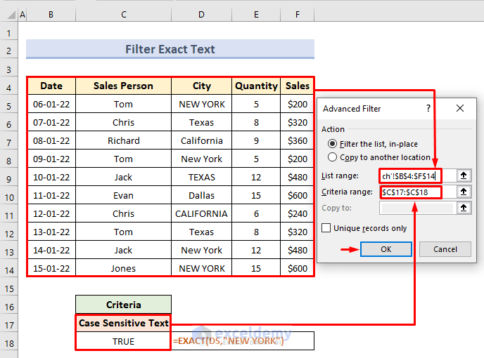
• Select the following filter criteria range: List Range: B4:F14, Criteria Range: C17:C18.
• Hit OK.

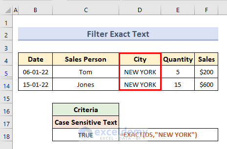
• We will get only the data for NEW YORK.

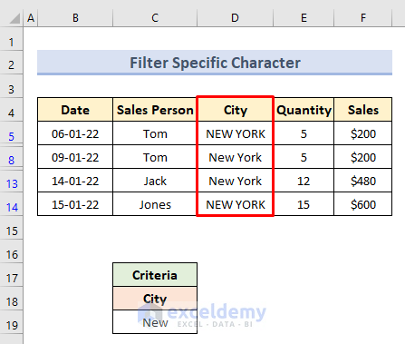
Case 2.1 – Having Specific Character at the Beginning

We will extract only the rows where the cities start with the word New.

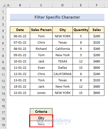
• Select the criteria ranges in the Advanced Filter box: List Range: B4:F14, Criteria Range: C18:C19.
• Press OK.

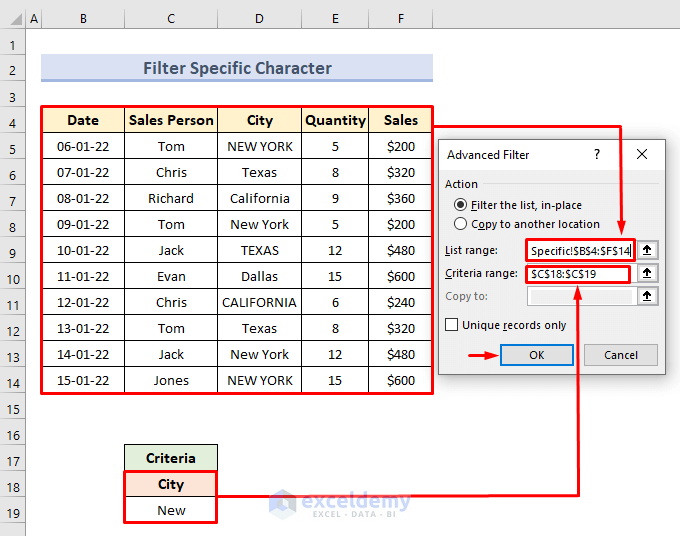
• We will get the data for all cities starting with the word New.

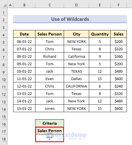
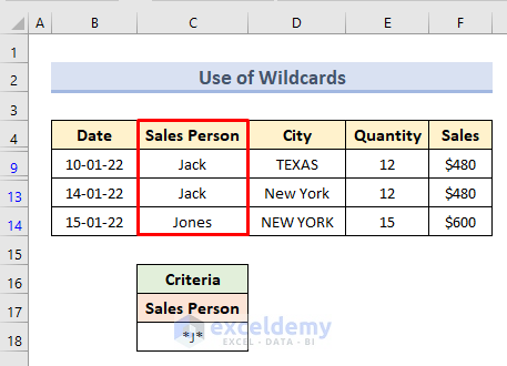
Method 3 – Use Wildcards with the Advanced Filter Option

Usually, there are three types of wildcard characters in Excel:

? (Question Mark) – Represents any single character in a text.

* (Asterisk) – Represents any number of characters.

~ (Tilde) – Represents the presence of a wildcard character in the text.

We’ll find the names of salespeople starting with the text J.

• Open the Advanced Filter window.
• Select the following criteria range: List Range: B4:F14, Criteria Range: C17:C18.
• Press OK.

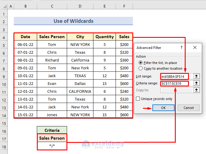
• We will get the names of salespeople that start with text J.

Method 4 – Apply a Formula with the Advanced Filter Criteria Range

We will extract the sales amounts greater than $350.

• Select cell C19.
• Insert the following formula:

• Hit Enter.

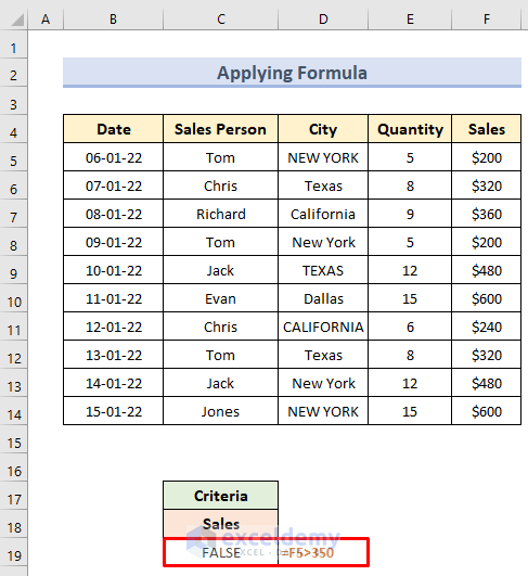
• The checks whether the sales value is higher than $350.

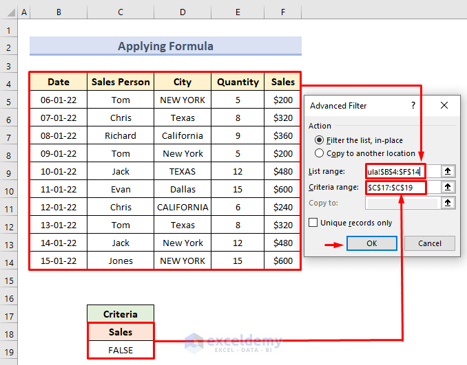
• Select the following criteria range in the Advanced Filter dialogue box: List Range: B4:F14, Criteria Range: C17:C19.
• Press OK.

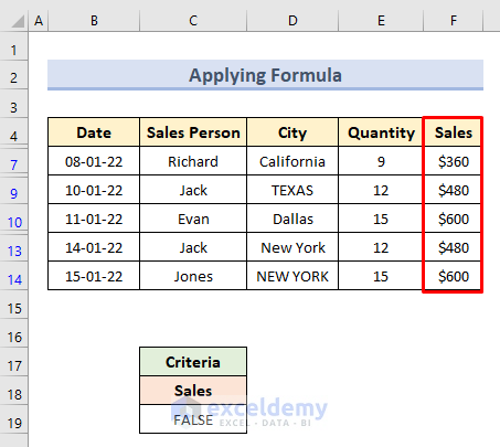
• We can see the data only where the sales are greater than $350.

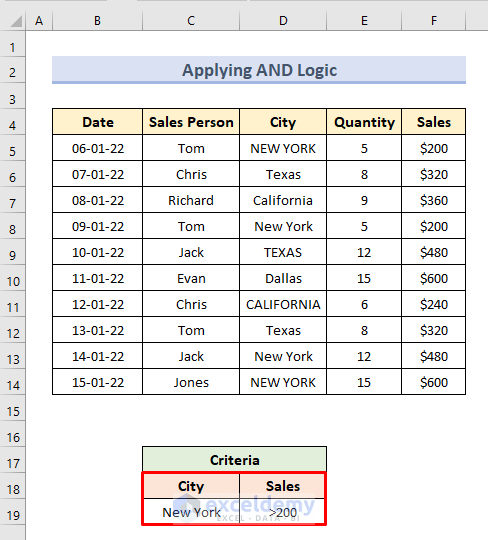
Method 5 – Advanced Filter with AND Logic Criteria

We have the following dataset. We will filter data for the city of New York and sales value >= 200.

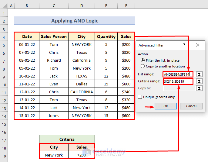
• Go to the Advanced Filter dialogue box and select the following criteria range: List Range: B4:F14, Criteria Range: C18:C19.
• Press OK.

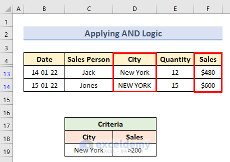
• Here are the results.

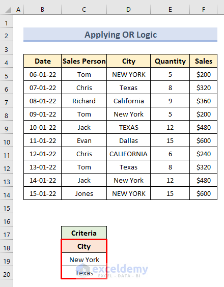
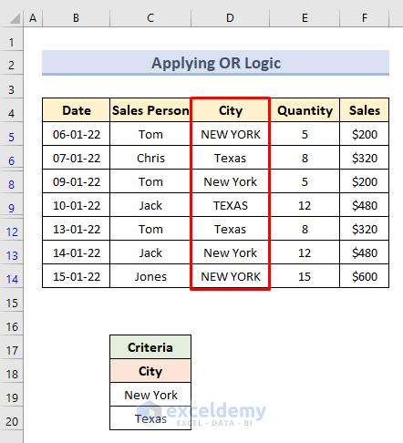
Method 6 – Using OR Logic with Advanced Filter Criteria Range

We will fetch data for New York and Texas.

• Open the Advanced Filter dialogue box.
• Input the following criteria range: List Range: B4:F14, Criteria Range: C18:C20.
• Hit OK.

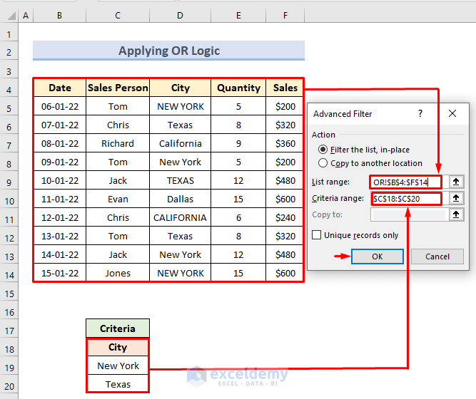
• We’ll get the filtered dataset for New York and Texas.

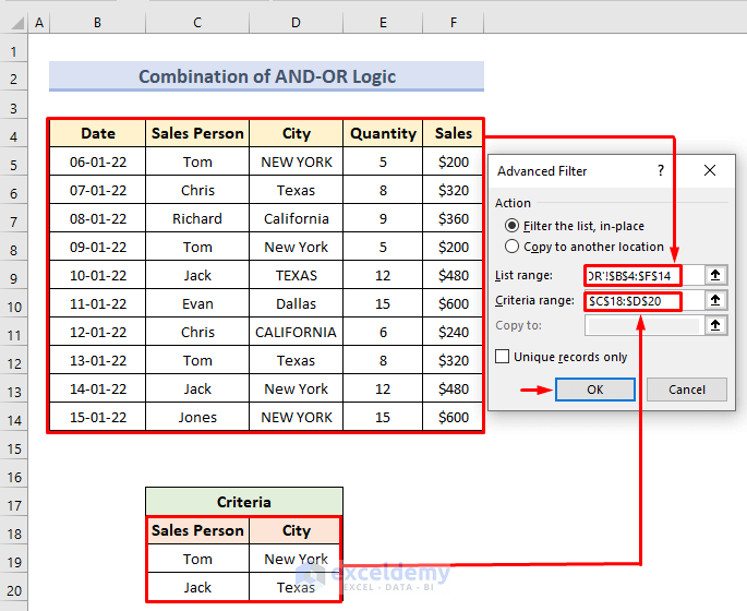
Method 7 – Combination of AND and OR Logic as Criteria Range

We will extract data from the following dataset based on multiple criteria, which are in the smaller table below.

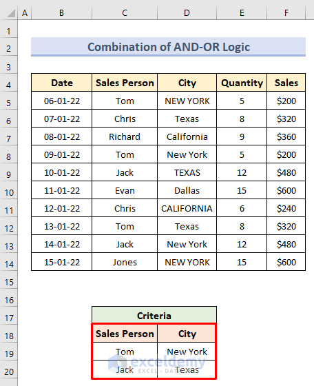
• Open the Advanced Filter dialogue box.
• Select the following criteria: List Range: B4:F14, Criteria Range: C18:C20.
• Then press OK.

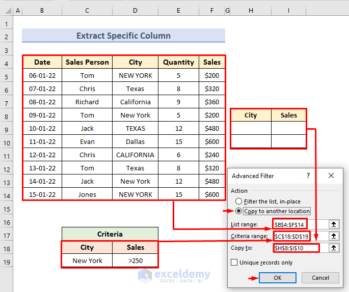
Method 8 – Using the Advanced Filter Criteria Range to Extract Specific Columns

After filtering, we will move the filtered part into another column.

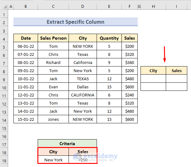
• From the Advanced Filter dialogue box, select the following criteria: List Range: B4:F14, Criteria Range: C18:C20.
• Select copy to another location option.
• In Copy to range, put H8:I10.
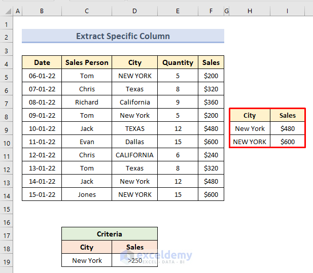
• Hit OK.

• We get the filtered data in H8:I10 according to our criteria.

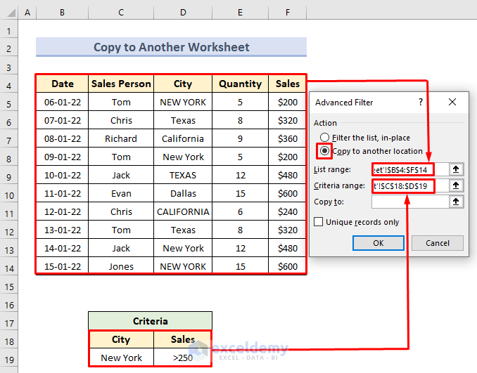
Method 9 – Copy Data to Another Worksheet after Filtering

• Go to the Another Worksheet-2 sheet where we will copy data after filtering.

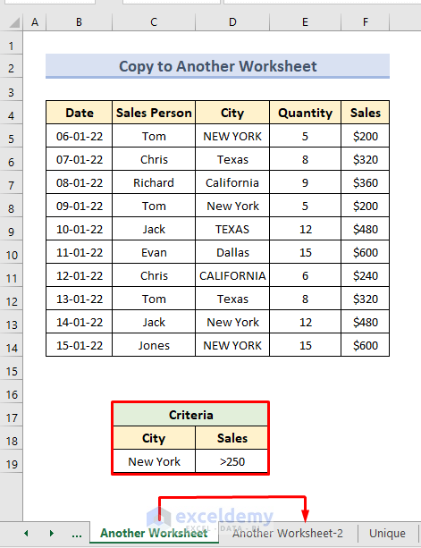
• We can see two columns, City and Sales, in Another Worksheet-2.

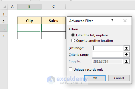
• Open the Advanced Filter dialogue box.

• Go to Another Worksheet-1.
• Select the following criteria: List Range: B4:F14, Criteria Range: C18:C19.
• Select the copy to another location option.

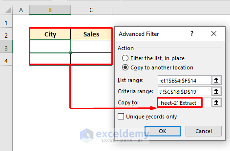
• Go to Another Worksheet-2.
• For Copy to range, put B2:C4.
• Press OK.

• We can see the filtered data in Another Worksheet-2.

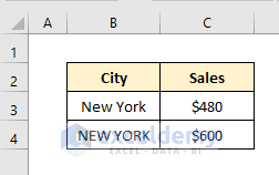
Method 10 – Extract Unique Records with Advanced Filter Criteria

We will extract unique values of cities in another column.

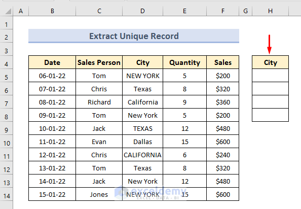
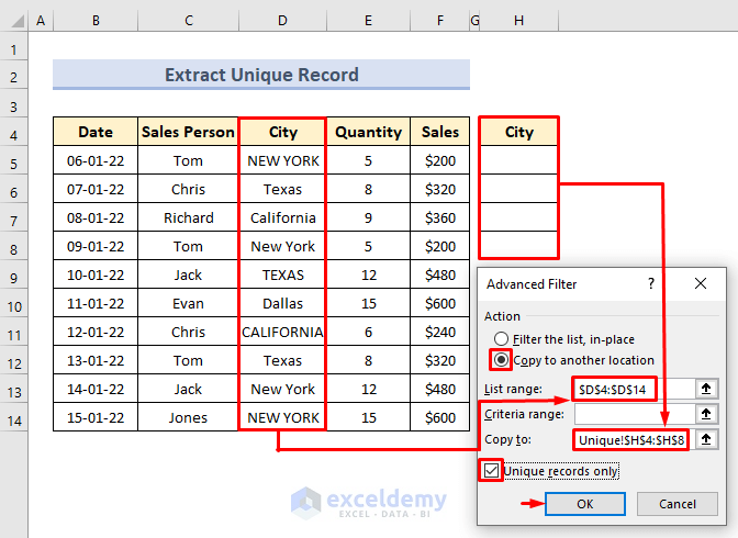
• Open the Advanced Filter window. Select the criteria List range: D4:D14.
• Select the option Copy to another location.
• Input the Copy to range as H4:H8.
• Check the box Unique records only.
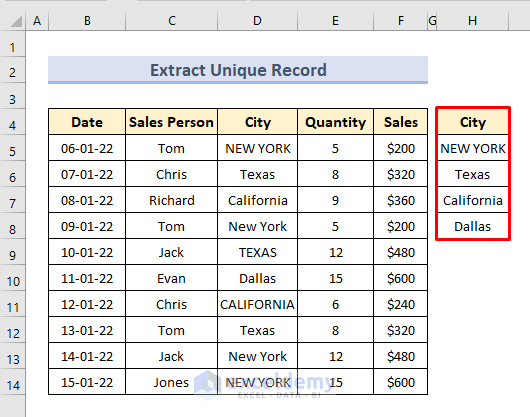
• Press OK.

• Here are the results.

Method 11 – Find Weekdays with the Advanced Filter Criteria Range

• Select cell C19.
• Insert the following formula:

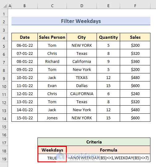
• Set the following criteria range in the Advanced Filter dialogue box: List Range: B4:F14, Criteria Range: C18:C19.
• Press OK.

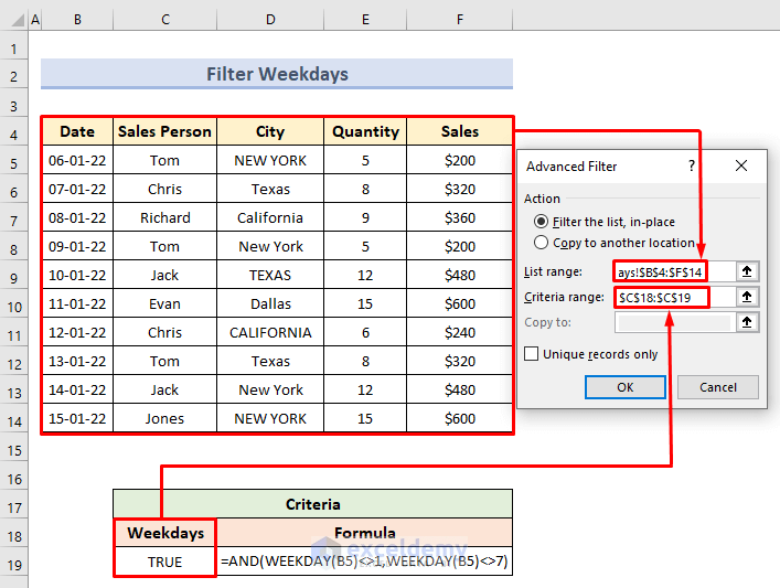
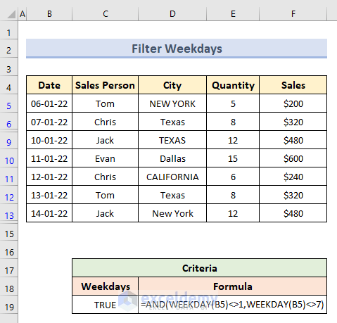
• We will get the Date values only for weekdays.

How Does the Formula Work?

• WEEKDAY(B5)<>1: 1 denotes Sunday. This part sets the criteria that the date is not Sunday.
• WEEKDAY(B5)<>7: 7 denotes Sunday. This part sets the criteria that the date is not Saturday.
• AND(WEEKDAY(B5)<>1,WEEKDAY(B5)<>7): Sets the criteria that the day is neither Saturday nor Sunday.

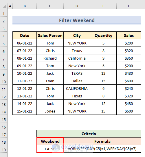
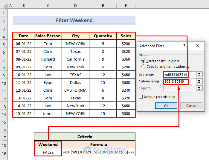
Method 12 – Apply Advanced Filter to Find the Weekend

• Select cell C19.
• Insert the following formula:

• Press Enter.

• From the Advanced Filter dialog box, select the following criteria range: List Range: B4:F14, Criteria Range: C18:C19.
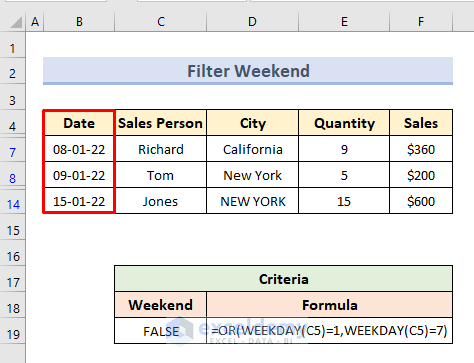
• Press OK.

• We can see only the values of the weekend in the Date column.

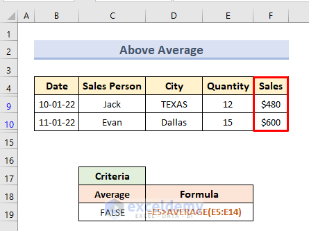
Method 13 – Use the Advanced Filter to Calculate Values Below or Above Average

We will only filter the sales value which is greater than the average sales value.

• Select cell C19.
• Insert the following formula:

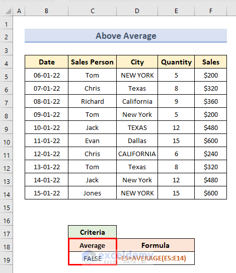
• Open the Advanced Filter dialogue box. Input the following criteria range: List Range: B4:F14, Criteria Range: C18:C19.
• Press OK.

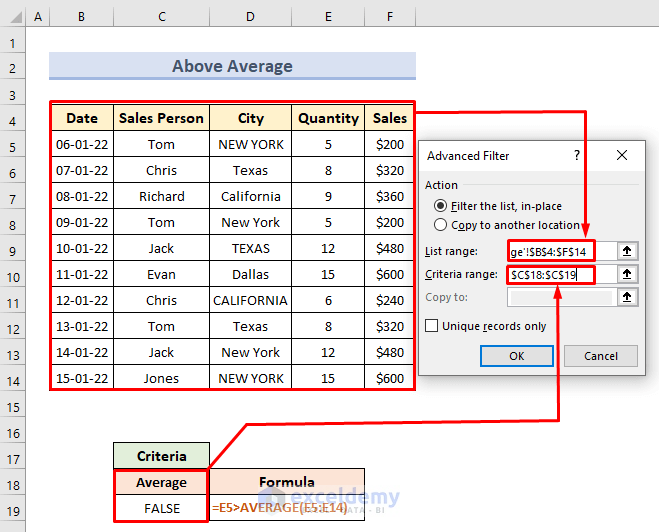
• We get only the dataset for sales value greater than the average value.

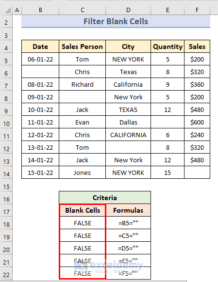
Method 14 – Filtering Blank Cells with OR Logic

• We have set the criteria by using the following formula type:

• We repeated this formula for each column (B through F) and put it in the range C18:C22.

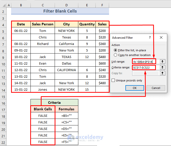
• Go to the Advanced Filter dialogue box.
• Input the following criteria: List Range: B4:F14, Criteria Range: C17:C22.
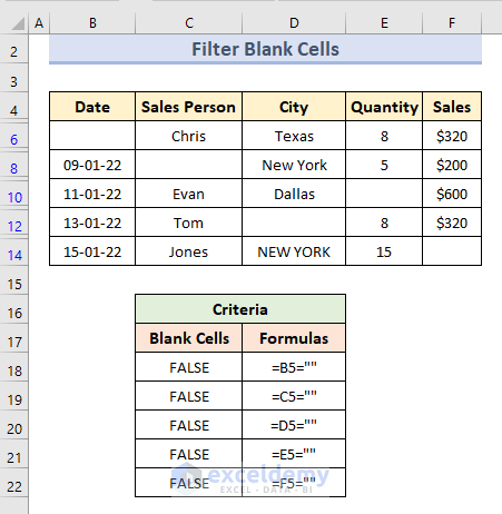
• Press OK.

• We get the dataset that only consists of rows with some blank cells.

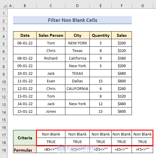
Method 15 – Apply the Advanced Filter to Filter Non-Blank Cells using OR as well as AND Logic

We will show only rows without any blank cells.

• We have set the following criteria for using the formula:

• We repeated this for each column.

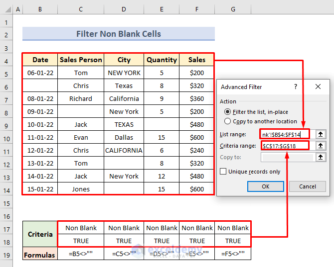
• Go to the Advanced Filter dialogue box.
• Insert the following criteria range: List Range: B4:F14, Criteria Range: C17:G18
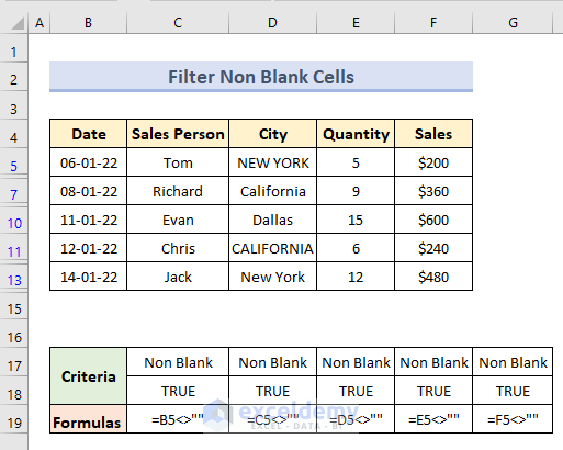
• Press OK.

• We get the filtered dataset.

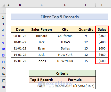
Method 16 – Find Top 5 Records Using the Advanced Filter Criteria Range

We will take the first five values of the Sales column.

• Use the following criteria formula:

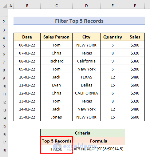
• Go to the Advanced Filter dialogue box.
• Insert the following criteria range: List Range: B4:F14, Criteria Range: C17:C18.
• Hit OK.

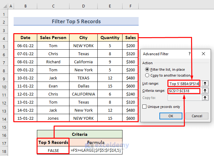
• We get the top five records of the Sales column.

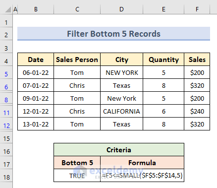
Method 17 – Use the Advanced Filter Criteria Range to Find the Bottom Five Records

• To find the bottom five records for the Sales column, we will use the following formula:

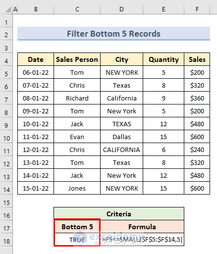
• Insert the following criteria range in the Advanced Filter dialogue box: List Range: B4:F14, Criteria Range: C17:C18.
• Press OK.

• We can see the bottom five values of the Sales column.

Method 18 – Filter Rows According to a List’s Matching Entries Using the Advanced Filter Criteria Range

Case 18.1 – Matches with Items in a List

We will take only the matching entries between the city columns.

• Here’s the criteria formula:

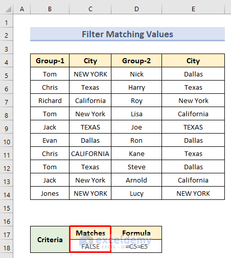
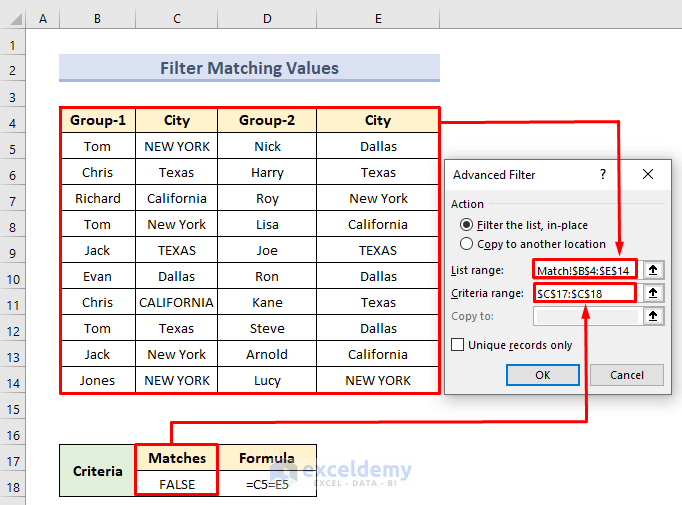
• Open the Advanced Filter option.
• Insert the following criteria range: List Range: B4:F14, Criteria Range: C17:C18.
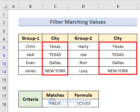
• Hit OK.

• We can see the rows that have the same value in the city columns.

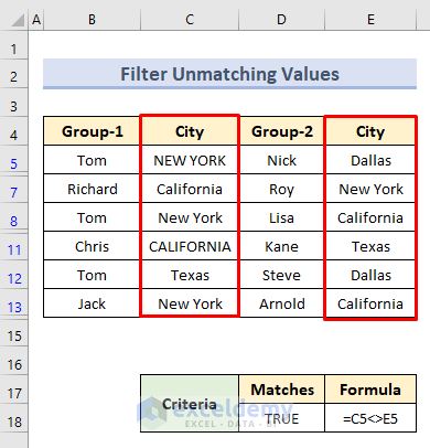
Case 18.2 – Distinct Items

• We will set the criteria by using the following formula:

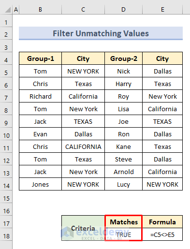
• From the Advanced Filter, insert the following criteria range: List Range: B4:F14, Criteria Range: C17:C18.
• Press OK.

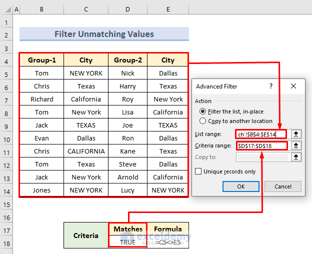
• We will get filtered rows where the values of cities in Column C and Column E do not match with one another.

Download the Practice Workbook

<< Go Back to Advanced Filter | Filter in Excel | Learn Excel