How to Create Dynamic Advanced Filter in Excel: 2 Applications

Method 1. Dynamic Advanced Filter with a Keyboard Shortcut Created by Using Excel Macros

Steps:

• In the Code section from the Developer tab, you will find an icon for Record Macro.

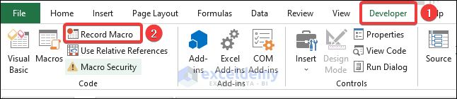
• Click that.

A new dialog box will pop up.

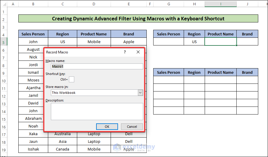
• Provide the Macro a name, your desired shortcut key, and the scope of the Macro.
• We have provided the macro name as Advanced_Filter. And have chosen CTRL + SHIFT + P as the shortcut key.

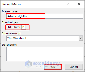
• Keep in mind the CTRL key is mandatory & Excel will automatically start the shortcut with this key.
• Repeat the process of what we have done in the Basic of Advanced Filter section.
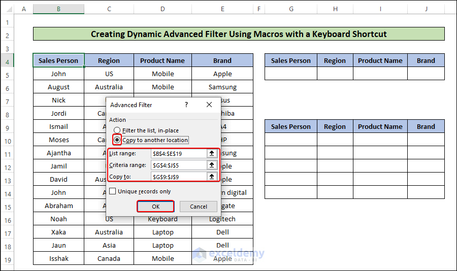
• Choose the Advanced option from the Sort & Filter.

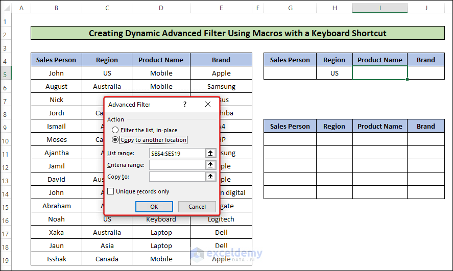
• Select the List range, Criteria range, and Copy to. Click OK.
• We did the same as previously and our result is also the same.

• From the Developer tab click Stop Recording. This will stop recording and save the Macro.

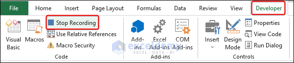
• Once we started recording the Macro, the icon changed to stop.
• Insert new criteria value and press CTRL + SHIFT + P (our chosen shortcut)

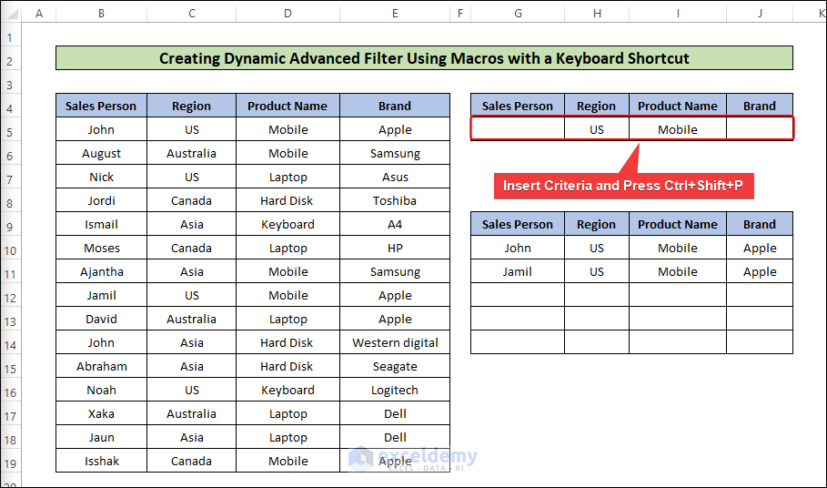
• We no longer repeat the process from the beginning. Just press the key.  And this will provide the desired outcome.

Method 2 – Dynamic Advanced Filter Button Created by Using Macros

Steps:

• In the Controls section of the Developer tab, there is an option called Insert. Click that. 

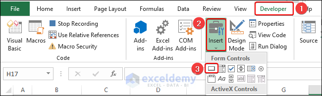
• Now from here select the Button. A dialog box will appear where you need to assign a Macro for the Button.
• This dialog box will open when you click Button. You need to name your Macro or create a new Macro.

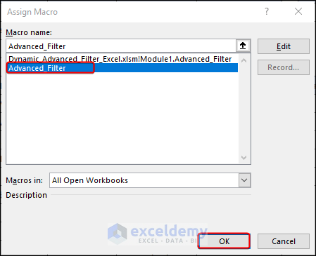
• We have a Macro Advanced_Filter, we have inserted that here. You can do that, or you can record a new Macro. Then click OK.

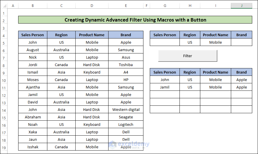
• We have named our Button as Filter. Feel free to set your preferred name.
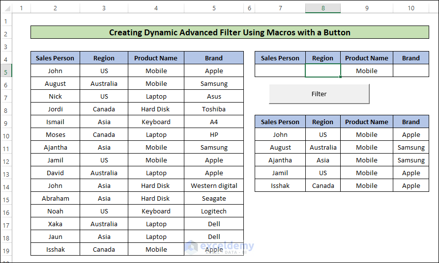
• Let us filter only by the product Mobile. Write the criteria value in the respective field. Click the button.

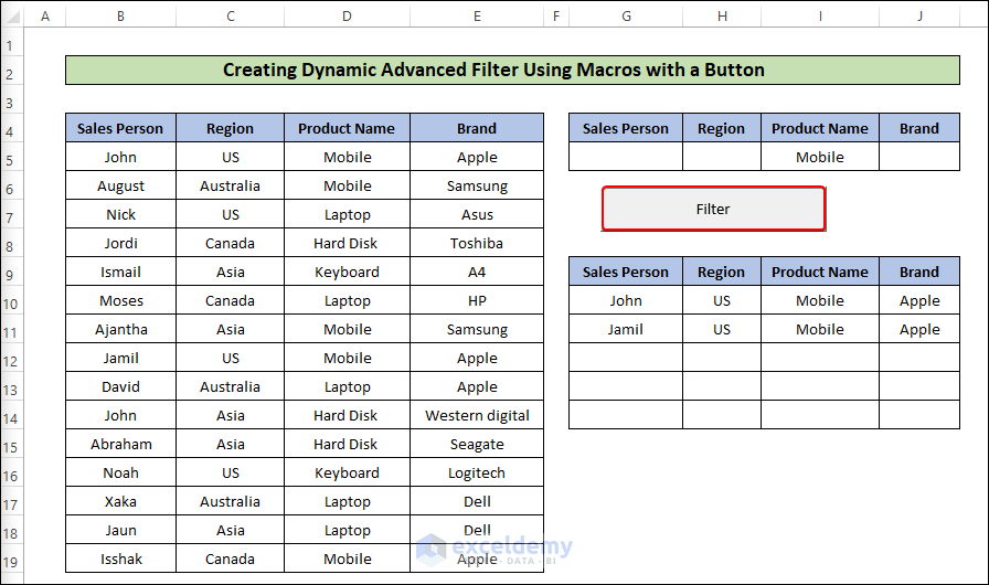
• We inserted Mobile in the Product Type column and clicked the button Filter. We found all the rows that contain Mobile irrespective of their region or brand.

How to Apply a Dynamic Filter in Excel

Steps:

• We will make the dynamic filter using the VBA code.
• We need to format our table by using the Format as Table.

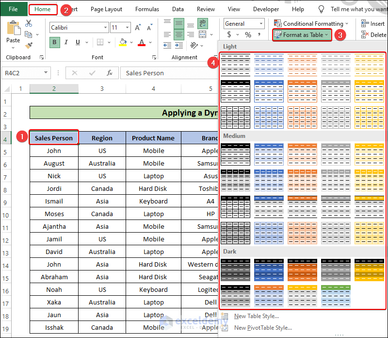
• Select any of the formats from here.

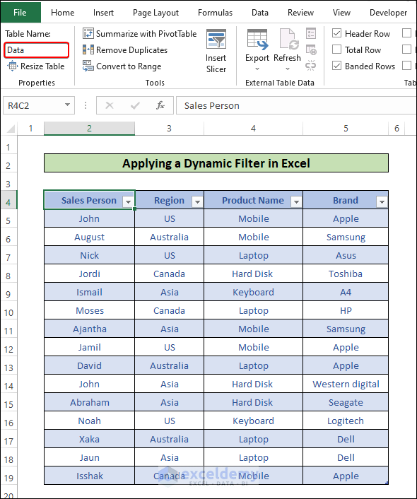
• Make sure to provide your table with a name. Here we have provided the table name as Data.
• From the Insert option of the Controls section within the Developer tab, select Text Box.

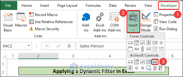
• Insert the box at your convenience.

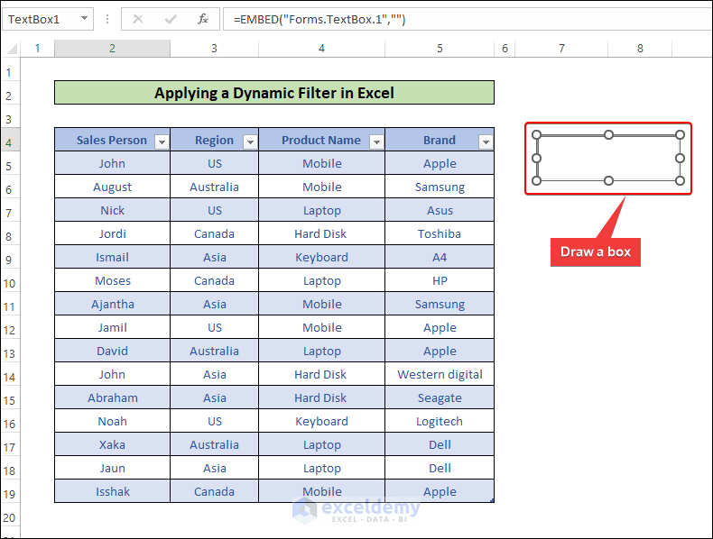
• You will be in the Design Mode similar to the image above. Double-click on the box. Microsoft Visual Basic for Application window will appear.

Copy and Paste the code there.
Private Sub TextBox1_Change()
Application.ScreenUpdating = False
ActiveSheet.ListObjects("Data").Range.AutoFilter Field:=2, Criteria1:= [G3] & "*", Operator:=xlFilterValues
Application.ScreenUpdating = True
End Sub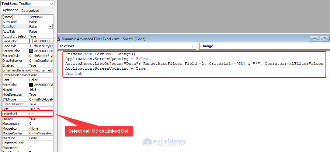

• In our code we have Criteria1:= [G3] & “*”, this is because what input we provide in the G3 cell will be our criteria. We have set G3 as our LinkedCell.
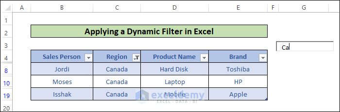
• [G3] & “*” means that our input should be at the first and then any value can be there.
• We have inserted Ca in the box and it returned values from the Canada region.

• Using Range.AutoFilter Field:=2 we have chosen the column Range. If you need other columns, change the number accordingly.

Download Practice Workbook

You can download the practice workbook from here:

<< Go Back to Advanced Filter | Filter in Excel | Learn Excel