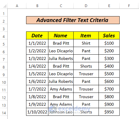
This is the sample dataset.
Method 1 – Using an Advanced Filter for a Cell That Contains Unique Text Values
The dataset contains duplicate values.
Steps:
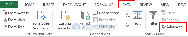
- Click the Data tab and choose Advance Filter or press ALT+A+Q
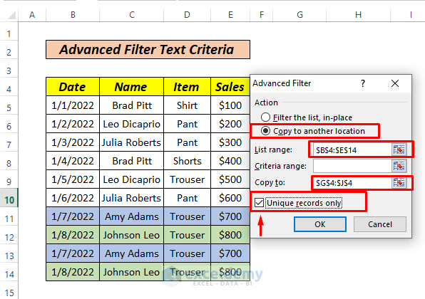
- In the dialog box, select Copy to another location.
- In List range, enter $B$4:$E$14.
- In Copy to, select a cell to copy the unique values.
- Check Unique records only.
- Click OK.
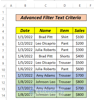
This is the output.
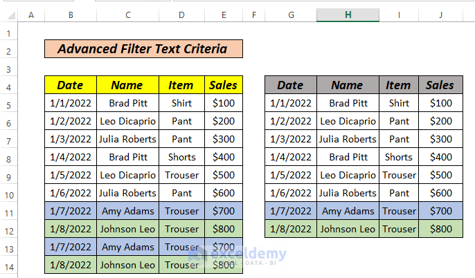
There are no duplicate values, only unique text records.
Method 2 – Using an Advanced Filter for Cells Whose Values are Exactly Equal to the Text Criteria
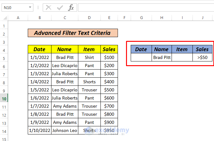
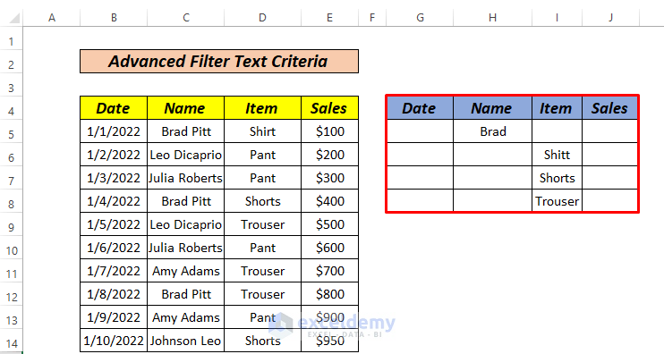
To extract data for a name that contains Brad and has a Sales value greater than $50.
Steps:
- Create a similar dataset, as shown below.
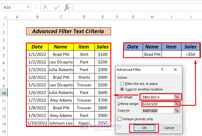
- In the dialog box, select Copy to another location.
- In List range, enter $B$4:$E$14.
- Enter the Criteria range.
- In Copy to, select a cell.
- Click OK.
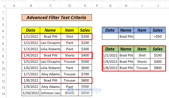
This is the output.
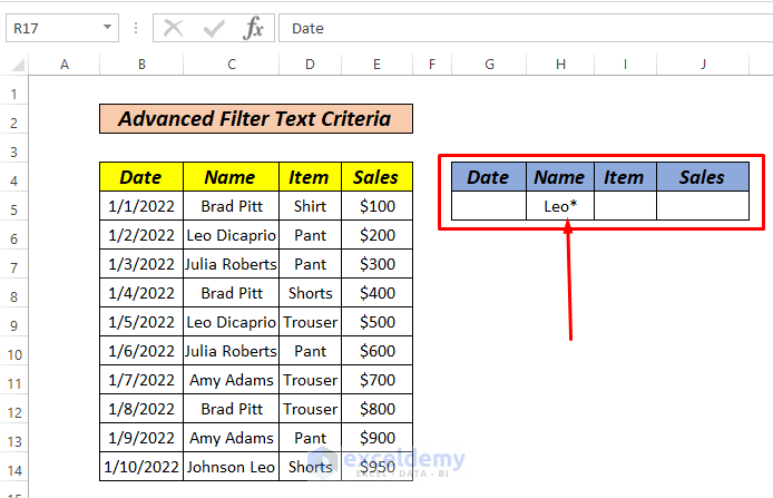
Method 3: Using an Advanced Filter for Text Values with Wildcard Characters
3.1: Filter Cells That Begin with a specific Text
To extract names that begin with Leo.
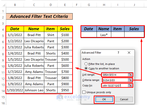
Steps:
- Create a similar dataset, as shown below.
- Select Copy to another location.
- Enter the List Range.
- Enter the Criteria range.
- In Copy to, select a cell.
- Click OK.
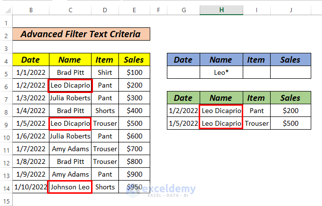
This is the output.
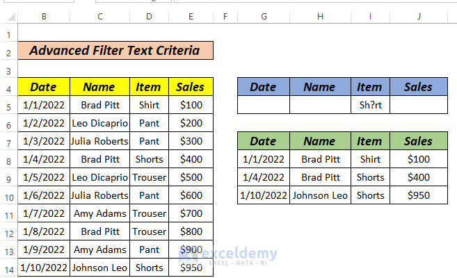
3.2: Filter Cells Using a Question Mark
Filter the items that start with Sh, have another letter after it and include rt.
Steps:
- Create a similar dataset, as shown below.
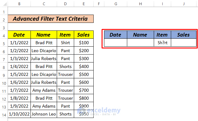
- Follow the steps described in Method 3.1.
This is the output.
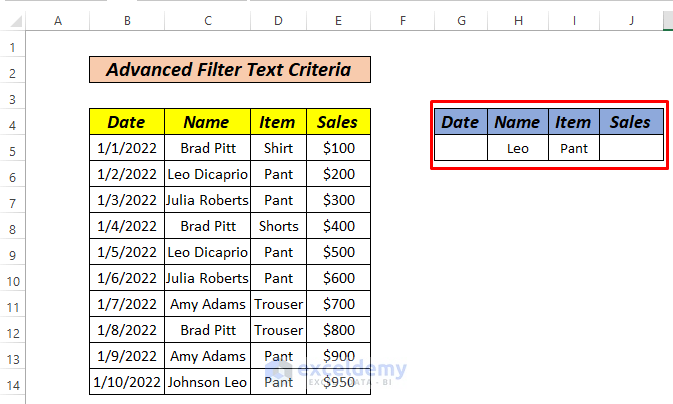
Method 4 – Using an Advanced Filter and the AND Rule for Text Values
Extract data with the name Leo and the item pant.
Steps:
- Create a similar dataset, as shown below.
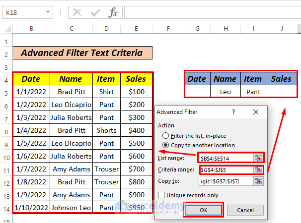
- Press ALT+A+Q.
- Select Copy to another location.
- Enter the List Range.
- Enter the Criteria range.
- In Copy to, select a cell.
- Click OK.
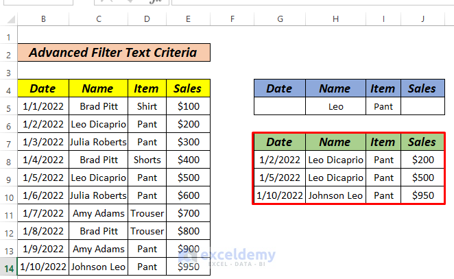
This is the output.
Method 5 – Using an Advanced Filter with the OR Rule for Text Criteria
Find the name Brad or the Items Shirt, Shorts or Trouser.
Steps:
- Create a similar dataset, as shown below.
- Follow the steps in Method 2.
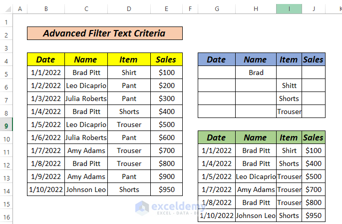
This is the output.
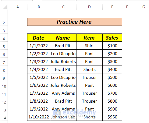
Practice Section
Practice here.
Download Practice Workbook
<< Go Back to Advanced Filter | Filter in Excel | Learn Excel
Get FREE Advanced Excel Exercises with Solutions!

Hi, I have two queries.
1. How to use advanced filter by the criteria of Date? I mean if I want to filter data of a certain month how can it be done by using advanced filter?
2. How to use advanced filter by the contains criteria? suppose if I want to filter data which contains ‘letter A’ or have ‘5’ how can it be done?
thank you.
Hi Shilpa, thanks for the response. Here’s the solution to your question no 1
You can simply create a criteria similar to the methods of this article using dates. Suppose you want to see the sales information after May. Please watch the following image for the process. I created the criteria in G6 cell.
In order to solve the second question of your comment, please apply the method described in the Section 3.2 of this article.
Hope this helps to solve your queries.
Hi, I have a query. If I want to leave out cells containing specific text using advanced excel, what criteria can I use? lets say, we want to have data excluding “pant”. I tried using (not equal to), but it doesn’t filter out. Please help
Hello Meghna Desai,
Great question. To exclude rows containing specific text like “pant” using Excel’s Advanced Filter, you can use the following setup in your criteria range:
If your column is called Item, then:
1. In the criteria range, use the same column header: Item
2. In the row below, enter this formula:
<>*pant*
This tells Excel to filter only rows not containing the word “pant”. The * is a wildcard, and <> means “not equal to”. So <>*pant* excludes any text that has “pant” anywhere in it.
Then apply the Advanced Filter as usual:
1. Go to the Data tab → Advanced (in the Sort & Filter group).
2. Set your List range and Criteria range.
3. Choose to filter in place or copy to another location.
Another Solution:
1. Add a new row above your data for criteria.
2. In the first cell of your criteria row (say, cell F1), type a different header than your data (e.g., Criteria).
3. In F2, enter the following formula (assuming your “Item” column is column C):
=ISERROR(SEARCH(“pant”, C2))
Then use the Advanced Filter, selecting this criteria range.
This formula will include only rows where “pant” is NOT found. The key is using SEARCH (to find “pant”) and wrapping it in ISERROR to exclude those matches.
Regards
ExcelDemy