Method 1 – Use Slicers to Filter Data from Worksheet
Steps:
- Select the whole dataset and choose the “Table” option from the “Insert” feature.
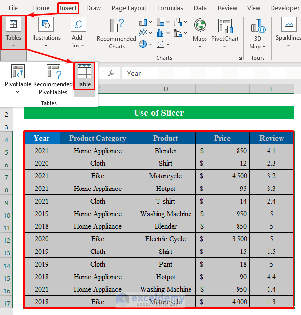
- Your dataset will be converted to a table.
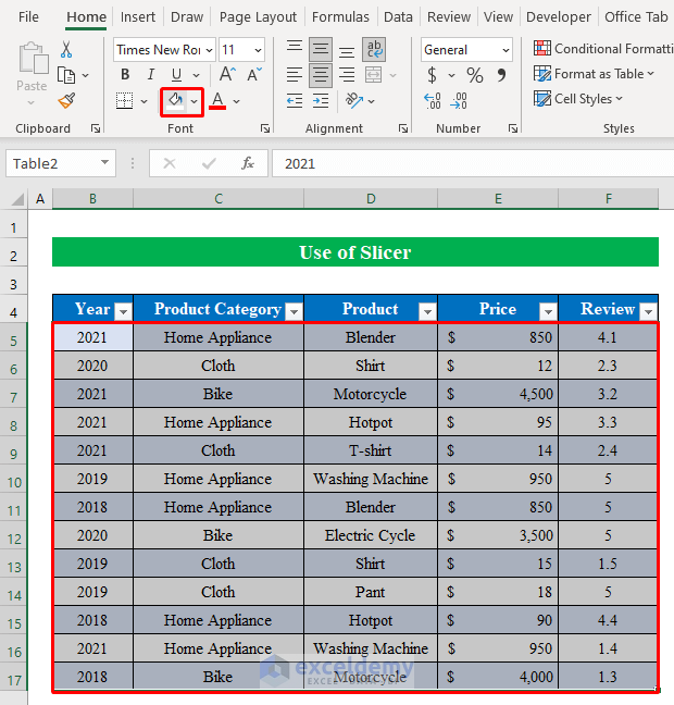
If you want you can change the background color.
- Select all the cells and changed the background color. We have selected “White”.
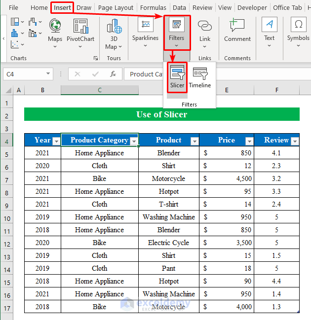
- Select any cell from the table, go to the “Insert” option and press “Slicer”.
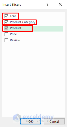
- From the new window, choose your filtering header and press OK.
- You will get all the slicers inside the worksheet.
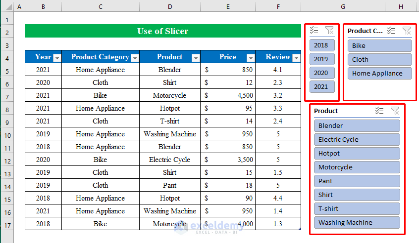
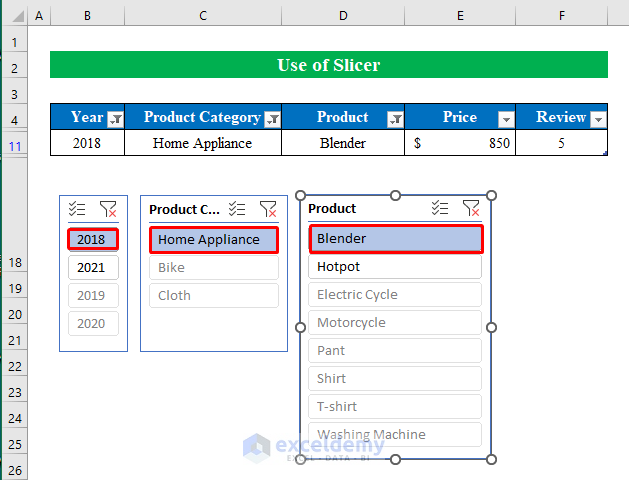
- To filter the data using the slicers, single click your desired “Year”, “Product Category”, and “Products” from the slicers and the dataset will visualize data according to it.
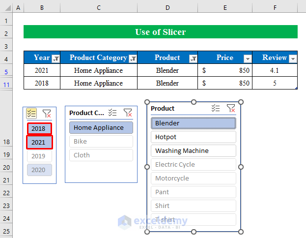
- You can also choose multiple filtering options from the slicers by clicking the “Multiple Selection” option at the top of any slicers.

- Click the “Multiple Selection” feature and choose various selections as shown in the image below.
Read More: How to Make Excel Slicer with Search Box
Method 2 – Apply Slicers to Filter Data in Pivot Table
Steps:
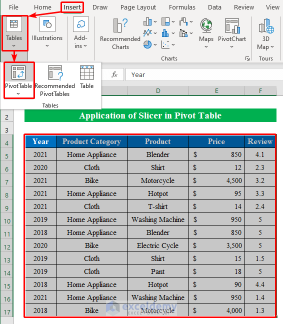
- Select the whole data from the table and choose “Pivot Table” from the “Insert” option.
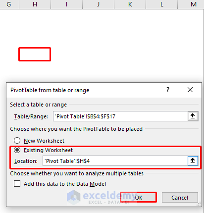
- From the new window, click the “Existing Worksheet” and choose a cell according to your choice in the worksheet.
- Press OK to continue.
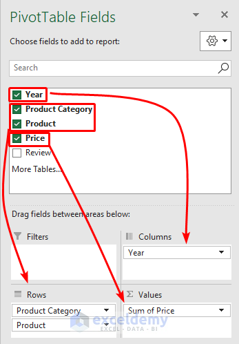
A right pane will pop up.
- Drag your headings to different locations to rearrange your pivot table.
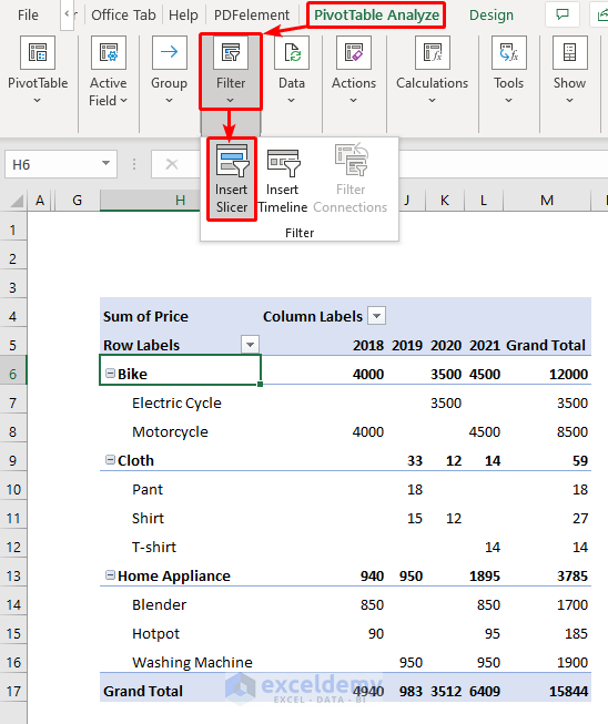
- Choose any cell from the pivot table and click the “Insert Slicer” option from the “PivotTable Analyze” feature.
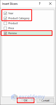
- Select any category from the list to open multiple slicers.
- Press OK to continue.
- You will get the chosen slicers for the pivot table.
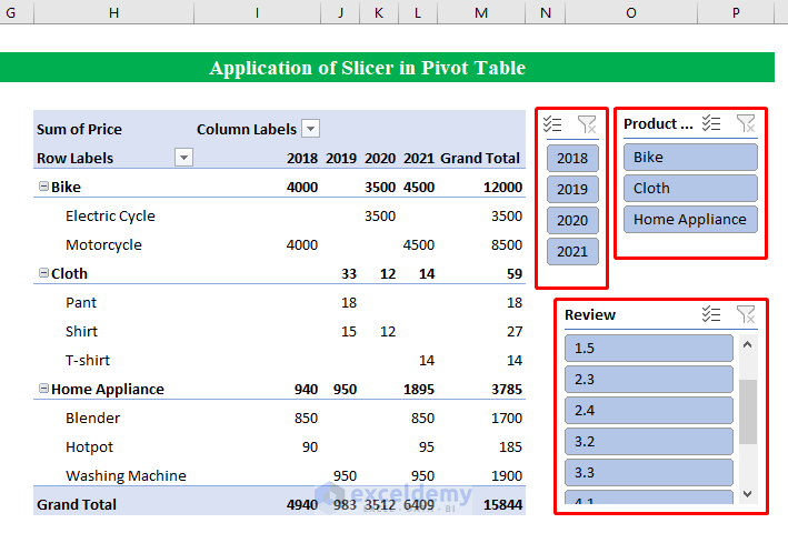
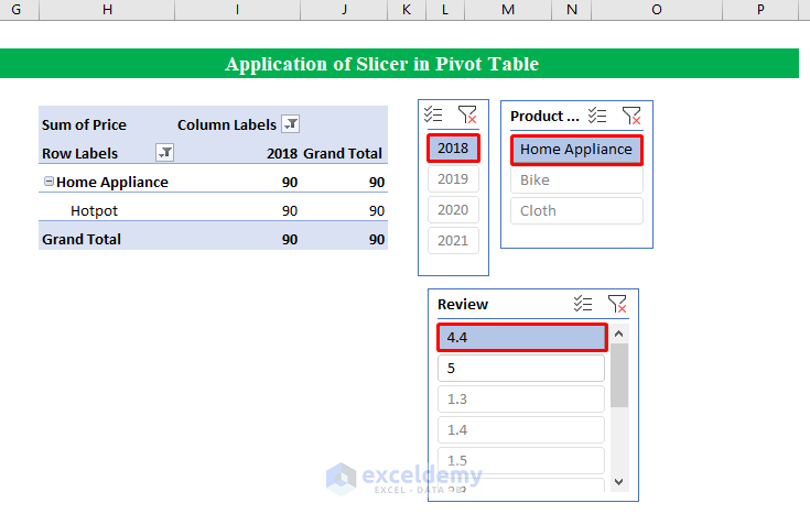
In the following image, we wanted to see the “Price” for the “Home Appliance” item sold in “2018” with a review of “4”.
Clicking the filters from multiple slicers we have the final output.
Download Practice Workbook
Further Readings
- How to Create Slicer Drop Down in Excel
- How to Custom Sort Slicer in Excel
- How to Group Dates in Excel Slicer
- Excel Slicer Vs Filter (Comparison & Differences)
- How to Create Timeline Slicer with Date Range in Excel

