The PRODUCT function is used to multiply numbers in Excel. Usually, you can multiply numbers using the product sign (*) in between numbers. But that method may not be convenient in all situations, especially when you need to work with lots of numbers.
The screenshot below is an overview of one of the applications of the PRODUCT function we will discuss in this article, and the dataset we’ll use to illustrate them.
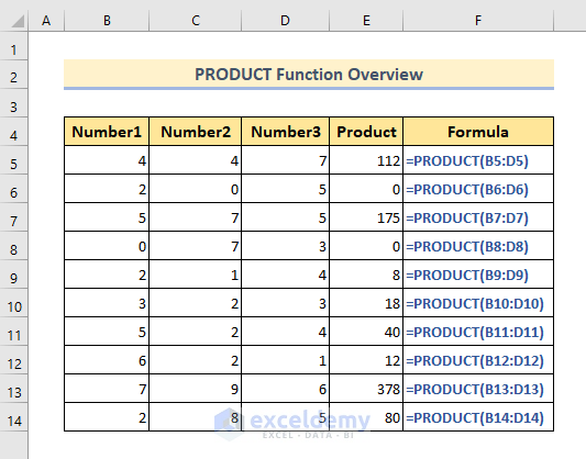
PRODUCT Function in Excel: Syntax
- Function Objective:
The PRODUCT function is used to calculate multiplication of numbers in Excel.
- Syntax:
=PRODUCT(number1, [number2], …)
- Arguments Explanation:
| Argument | Required/Optional | Explanation |
|---|---|---|
| number1 | Required | The first number of the range of numbers to be multiplied. |
| number2 | Optional | Extra numbers or range of numbers to be multiplied. |
- Return Parameter:
Multiplied value of the given numbers within the argument field.
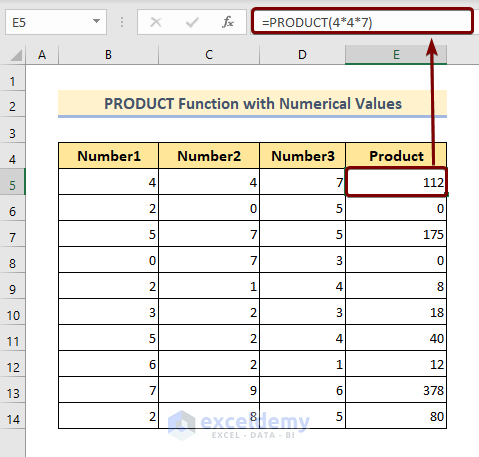
Example 1 – Using the PRODUCT Function with Numerical Values in Excel
We can use the PRODUCT function to multiply values in the traditional way, namely by putting the product sign (*) in between the numbers to be multiplied, for instance 5*8.
Steps:
- In cell E5, enter the following formula:
=PRODUCT(4*4*7)- Press ENTER.
The end result is as in the picture below:
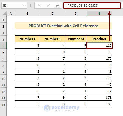
Example 2 – Using the PRODUCT Function with Cell References
To multiply values stored within cells, we specify the cell references separated by a comma inside the PRODUCT function argument field.
Steps:
- In cell E5, enter the following formula:
=PRODUCT(B5,C5,D5)- Press ENTER.
- Drag the Fill Handle icon to the end of the Product column.
The end result is as in the picture below:
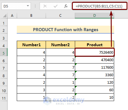
Example 3 – Using the PRODUCT Function with Numbers in Different Ranges
We can multiply multiple series of numbers, separated by a comma.
Steps:
- In cell E5, enter the following formula:
=PRODUCT(B5:B11,C5:C11)- Press ENTER.
- Drag the Fill Handle icon to the end of the Product column.
The end result is as in the picture below.
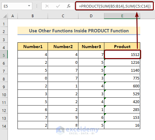
Example 4 – Combining SUM and PRODUCT Functions to Multiply Two or More Sums
Let’s multiply the sums of some ranges of numbers.
Steps:
- In cell E5, enter the formula within the cell:
=PRODUCT(SUM(B5:B14),SUM(C5:C14))- Press ENTER.
- Drag the Fill Handle icon to the end of the Product column.
The end result is as in the picture below:
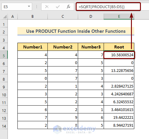
Example 5 – Finding the Square Root of a Product with SQRT and PRODUCT Functions
Steps:
- In cell E5, enter the following formula:
=SQRT(PRODUCT(B5:D5))- Press ENTER.
- Drag the Fill Handle icon to the end of the Product column.
The end result is as in the picture below:
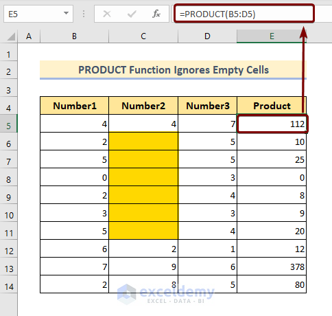
Example 6 – Using the PRODUCT Function with Ranges That Have Empty Cells
The PRODUCT function will ignore the blank cells within the specified range.
Steps:
- In cell E5, enter the following formula:
=PRODUCT(B5:D5)- Press ENTER.
- Drag the Fill Handle icon to the end of the Product column.
The end result is as in the picture below:
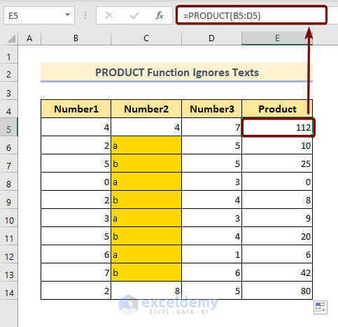
Example 7 – Using the PRODUCT Function with Text Values
The PRODUCT function will also ignore the cells containing text within the specified range, only counting cells containing numerical values.
Steps:
- In cell E5, enter the following formula:
=PRODUCT(B5:D5)- Press ENTER.
- Drag the Fill Handle icon to the end of the Product column.
The end result is as in the picture below:
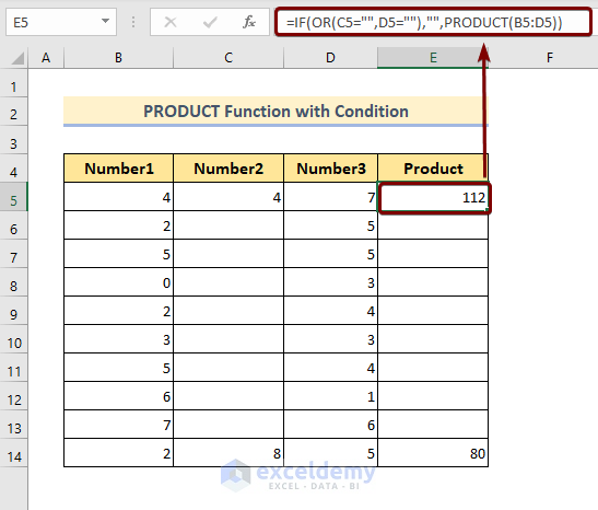
Example 8 – Using the PRODUCT Function to Multiply Data Based on a Condition
If we find a blank cell in a row, we want to exclude it from the calculation of the product of that row.
Steps:
- In cell E5, enter the following formula:
=IF(OR(C5="",D5=""),"",PRODUCT(B5:D5))- Press ENTER.
- Drag the Fill Handle icon to the end of the Product column.
The formula will return a blank cell if either of the values to be multiplied are blank, else it will return their product.
The end result as in the picture below:
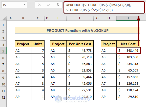
Example 9 – Using the PRODUCT Function to Multiply Two or More Outputs of the VLOOKUP Function
We can use the PRODUCT function along with the VLOOKUP Function.
Steps:
- In cell E5, enter the following formula:
=PRODUCT(VLOOKUP(H5,$B$5:$C$12,2,0), VLOOKUP(H5,$E$5:$F$12,2,0))- Press ENTER.
- Drag the Fill Handle icon to the end of the Product column.
The end result is as in the picture below:
Formula Breakdown:
- (VLOOKUP(H5,$B$5:$C$12,2,0) ▶ Looks for units in the table range B5:C12.
- VLOOKUP(H5,$E$5:$F$12,2,0) ▶ Looks for cost per unit in the table range E5:F12.
- =PRODUCT(VLOOKUP(H5,$B$5:$C$12,2,0), VLOOKUP(H5,$E$5:$F$12,2,0)) ▶ Multiples the number of unit and cost per unit returns from the two VLOOKUP functions.
Things to Remember
- You can insert a maximum of 255 arguments inside the PRODUCT function.
- If all the reference cells contain text, the PRODUCT function will return a #VALUE error.
Download the Practice Workbook
<< Go Back to Excel Functions | Learn Excel
Get FREE Advanced Excel Exercises with Solutions!

HI THERE!
4. Combining SUM and PRODUCT Functions to Multiply Two or More Sums
THIS EXAMPLE CASE IS UNABLE TO UNDERSTAND THE RESULTING VALUES.
WOULD REQUEST A CLARIFICATION WITH SLIGHTLY DEEPER INTERPRETATION….
Hello UMESH!
Thanks for reaching out and sharing your problem with us.
let’s break down the given formula =PRODUCT(SUM(B5:B14),SUM(C5:C14)) and provide a deeper interpretation:
SUM(B5:B14): calculates the sum of the values in the range from cell B5 to B14. It adds up all the numbers in that specified range.
SUM(C5:C14): calculates the sum of the values in the range from cell C5 to C14. It adds up all the numbers in that specified range.
=PRODUCT(SUM(B5:B14),SUM(C5:C14))
The outer PRODUCT function takes the results of the two SUM functions and multiplies them together. In other words, it multiplies the sum of values in range B5:B14 by the sum of values in range C5:C14.
When you AutoFill the above formula, it will automatically create relative cell references within a similar data range.
If you want to get the total product result in a single cell, use absolute cell references instead of relative cell references in the above formula. Then, use the following formula instead of the one above
=PRODUCT(SUM($B$5:$B$14),SUM($C$5:$C$14))
Again, thank you for being with us.
Regards
Md. Abdur Rahim Rasel
Exceldemy Team
Very Useful and helpful
Hello George Jululian,
You are most welcome.
Regards
ExcelDemy