This is an overview:
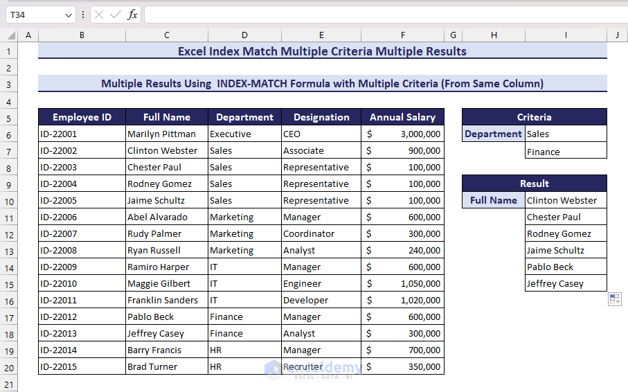
Method 1 – Get Multiple Results Using the INDEX-MATCH Formula Based on 2 Criteria (in the Same Column)
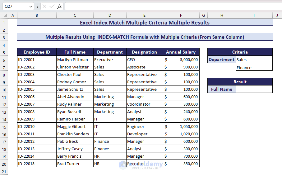
Consider the following dataset.
To find the list of employees from the Sales and Finance Department in the Full Name column:
Click the image for a detailed view
Steps:
- In I10, enter the following formula.
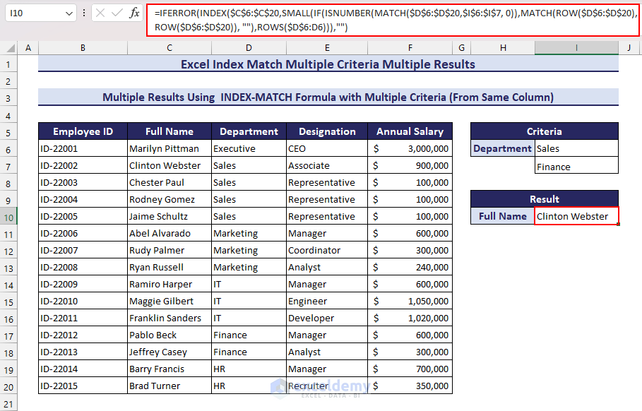
=IFERROR(INDEX($C$6:$C$20,SMALL(IF(ISNUMBER(MATCH($D$6:$D$20,$I$6:$I$7, 0)),MATCH(ROW($D$6:$D$20),ROW($D$6:$D$20)),""),ROWS($D$6:D6))),"")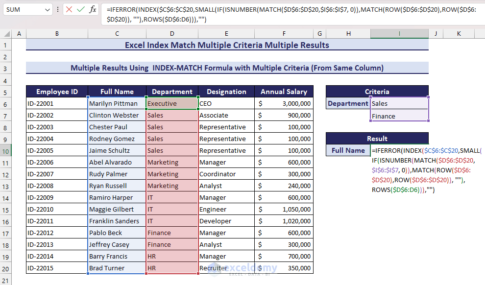
Click the image for a detailed view
- Press Enter to see the first match.
You can click the image for a detailed view
- Drag down the Fill Handle to see the result in the rest of the cells.
Click the image for a detailed view
- Drag down the Fill Handle icon to get all matched values for the given conditions.
Click the image for a detailed view
If you change the department names, the matched Full Names will also change.
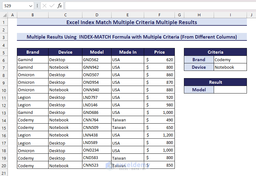
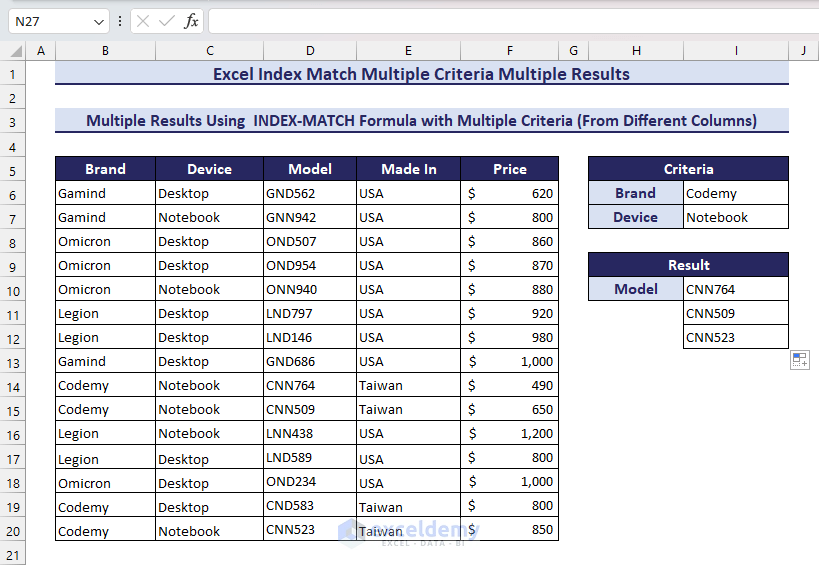
Method 2 – Getting Multiple Results with the INDEX-MATCH Formula Based on 2 Criteria (in Different Columns)
Consider the following dataset.
To see the list of Codemy Notebook Models:
You can click the image for a detailed view
Steps:
- Enter the following formula in I10.
=IFERROR(INDEX($D$6:$D$20, SMALL(IF(ISNUMBER(MATCH($B$6:$B$20, $I$6, 0)*MATCH($C$6:$C$20,$I$7,0)), MATCH(ROW($B$6:$B$20), ROW($B$6:$B$20)), ""), ROWS($D$6:D6))),"")- Press Enter.
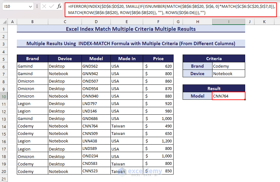
Click the image for a detailed view
- Drag down the Fill Handle to see the result in the rest of the cells.
You can click the image for a detailed view
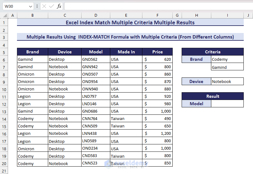
Method 3 – Getting Multiple Results with the INDEX-MATCH Formula Based on 3 Criteria
Find Gamind or Codemy Notebook models:
Click the image for a detailed view
Steps:
- Enter the following formula in I12.
=IFERROR(INDEX($D$6:$D$20, SMALL(IF(ISNUMBER(MATCH($B$6:$B$20, $I$6:$I$7, 0)*MATCH($C$6:$C$20,$I$9,0)), MATCH(ROW($B$6:$B$20), ROW($B$6:$B$20)), ""), ROWS($D$6:D6))),"")- Press Enter.
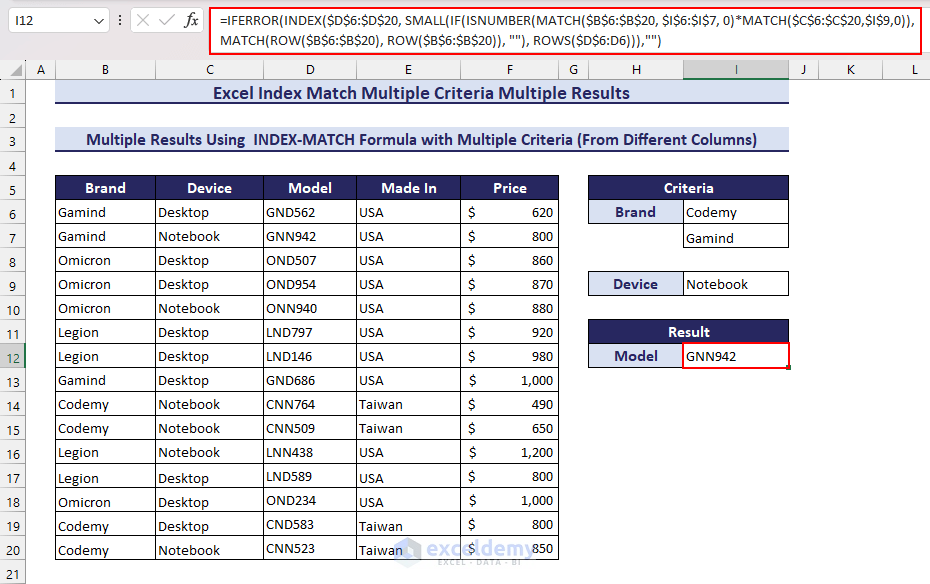
You can click the image for a detailed view
- Drag down the Fill Handle to see the result in the rest of the cells.
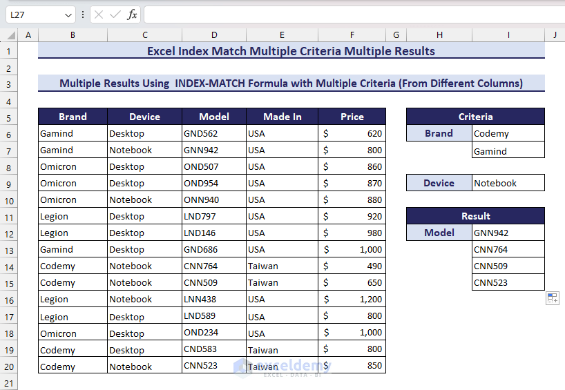
Click the image for a detailed view
Method 4 – Using the FILTER and the COUTNIF Functions
Consider the dataset used in Method 1.
- Use the following formula and press Enter.
=FILTER(C6:C20,COUNTIF(I6:I7,D6:D20))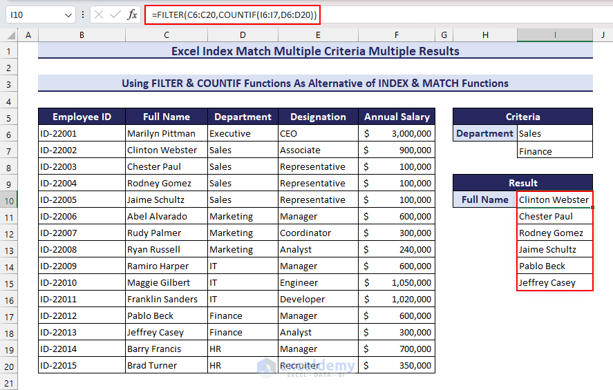
Click the image for a detailed view
Consider the dataset used in Method 2.
- Use the following formula.
=FILTER(D6:D20,(B6:B20=I6)*(C6:C20=I7))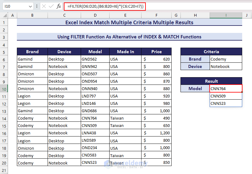
You can click the image for a detailed view
Download Practice Workbook
<< Go Back to Multiple Criteria | INDEX MATCH | Formula List | Learn Excel
Get FREE Advanced Excel Exercises with Solutions!

Hi,
In the array formula =INDEX($A$2:$A$14,SMALL(IF(ISNUMBER(MATCH($D$2:$D$14,$G$3,0)),MATCH(ROW($D$2:$D$14),ROW($D$2:$D$14)),””),ROWS($F$1:F1)))
What should I do if I need to add one more criteria, for example Country and Sex. Please help.
I have a condition where I need to match two (sometimes three) criterias and get multiple matching results.
Thanks in advance.
Hi Deepak!
The following formula can match two criteria and return multiple matches:
=INDEX($E$2:$E$14, SMALL(IF(COUNTIF($G$2, $C$2:$C$14)*COUNTIF($H$2, $D$2:$D$14), ROW($A$2:$E$14)-MIN(ROW($A$2:$E$14))+1), ROW(A1)), COLUMN(A1))Here,
$E$2:$E$14= Column to return matches$G$2 and $H$2= Criteria 1 and 2$C$2:$C$14and$D$2:$D$14= The columns of main data respective to criteria 1 and 2In a similar way, you can add any number of criteria.
Thank you for being with us.
Hi,
Can you show me the formula if you change the criteria to dates?
Hello KYLE,
Obviously, you can do that for dates also. See the image below.
Here, we retrieved the Price of a product with 2 criteria. One is the Product Name, another criterion is the date. The formula we used in cell I5 is the following.
=INDEX($E$5:$E$16,MATCH(1,(($B$5:$B$16=G5)*($D$5:$D$16>=H5)*($C$5:$C$16<=H5)),0))You can go through the article How to Use INDEX MATCH with Multiple Criteria for Date Range on our website for an explanation of this formula and other methods to do the same task.
Anyway, I hope that helps. You may follow our website, ExcelDemy, a one-stop Excel solution provider, to explore more. Happy Excelling.
Regards,
Shahriar Abrar Rafid
Excel & VBA Content Developer
ExcelDemy
Sir, kindly explain the last part of this formula – =INDEX($B$4:$F$17,MATCH($I$5,($B$4:$B$17),0),ROW()-6)
I mean the ROW ()-6
Thanks in advance.
Hello OLAWANDE,
I get your question. It’s a pleasure to us that our readers read our content well and ask us questions if they don’t get it. Also, they give us positive feedback. Thanks, OLAWANDE.
Now, getting back to your query. You wanted to know the purpose of ROW()-6 in this formula. To understand it, you have to have a clear concept of the INDEX function and its arguments. Syntax of the INDEX function in array form is like the following.
=INDEX(array, row_num,[column_num])If you match this structure with the formula, you can easily perceive that ROW()-6 is the column_num argument of the INDEX function.
Now, look at the worksheet. At first, we want to get the Age of this person. The output range is in Row 8. So, for cell I8, the ROW function will return us 8. After that, subtracting 6 from this, we get 2. Then, look at the array which is B4:F17. In this array, which column contains the Ages?? Obviously, the second column. That’s how ROW()-6 gives us the column number to match in the array.
Similarly, to find the Sex in cell I9, we used the same formula. Here, ROW()-6 returns us 3. And the 3rd column of the array contains the Sex of the people.
I think you understood now, how this part of the formula works. Thanks again for your beautiful comment. You may visit our website, ExcelDemy, a one-stop Excel solution provider, to explore more.
Regards,
Shahriar Abrar Rafid
Excel & VBA Content Developer
Team ExcelDemy
Howdy.
Is it possible to use wildcards with the second formula?
=INDEX($B$5:$B$17, SMALL(IF(COUNTIF($F$6, $C$5:$C$17)*COUNTIF($G$6, $D$5:$D$17), ROW($B$5:$D$17)-MIN(ROW($B$5:$D$17))+1), ROW(A1)), COLUMN(A1))
Hi ALLISON,
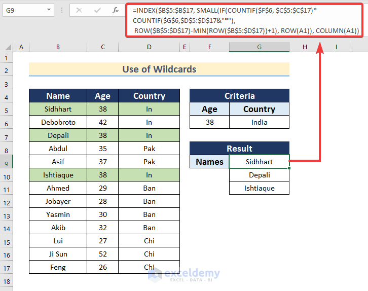
If you want to use wildcards with the second formula, you need to modify the dataset a little bit. Let’s say, we have short form of country name in the “Country” column. Our aim is to find the name of the person aged “38” and whose country is “India“. You can use the following formula:
=INDEX($B$5:$B$17, SMALL(IF(COUNTIF($F$6, $C$5:$C$17)*COUNTIF($G$6,$D$5:$D$17&”*”),ROW($B$5:$D$17)-MIN(ROW($B$5:$D$17))+1), ROW(A1)), COLUMN(A1))
We have used the wildcards character ampersand (*) in the second COUNTIF portion: COUNTIF($G$6,$D$5:$D$17&”*”)
As we want to find multiple output so it will result from an array. So, the $D$5:$D$17 acts as criteria as we can use wildcards character in criteria. This formula will match the short form mentioned in the country column and match it with criteria and extract the Name.
Hope you find this helpful.
Regards
Rafiul Hasan
Team ExcelDemy
Good Day, Would one be able to display the results horizontally (across a row) as opposed to vertically (down the column)
Hi John,
Thanks for your comment. Follow the below procedures for your purpose:
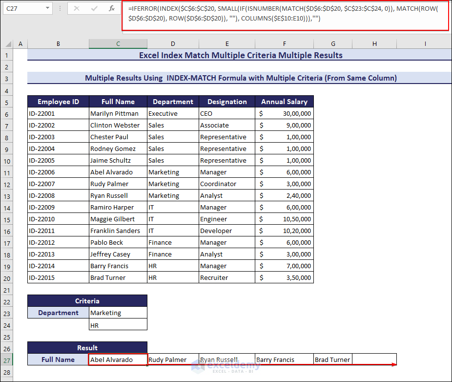
1. Get Multiple Results Using INDEX-MATCH Formula Based on 2 Criteria from the Same Column
Insert the following formula for the same case given in the article but to get values horizontally. After inserting formula in cell C27, drag the fill handle icon till it gives blank results.
=IFERROR(INDEX($C$6:$C$20, SMALL(IF(ISNUMBER(MATCH($D$6:$D$20, $C$23:$C$24, 0)), MATCH(ROW($D$6:$D$20), ROW($D$6:$D$20)), “”), COLUMNS($E$10:E10))),””)
2. Get Multiple Results Using INDEX-MATCH Formula Based on 2 Criteria from Different Columns
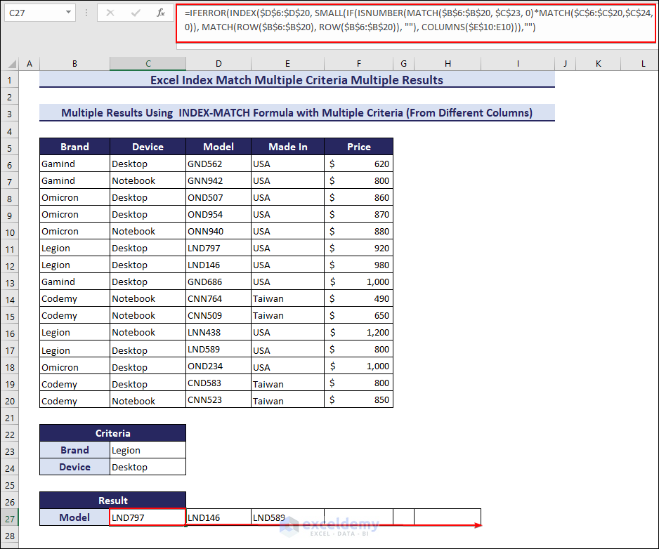
Similary for getting multiple results based on 2 criteria from different columns for same case given in the article but in horizontal direction, insert the following formula in cell C27 and drag the fill handle icon till it gives blank results.
=IFERROR(INDEX($D$6:$D$20, SMALL(IF(ISNUMBER(MATCH($B$6:$B$20, $C$23, 0)*MATCH($C$6:$C$20,$C$24,0)), MATCH(ROW($B$6:$B$20), ROW($B$6:$B$20)), “”), COLUMNS($E$10:E10))),””)
You can download the modified workbook from this link for your purpose. Hope, your problem will be solved. If not, share with us in the reply or you can share your workbook in ExcelDemy Forum.
Best Regards,
ExcelDemy Team