You can implement an Excel statistical function while using a dataset. At times, you need to know the largest value in multiple ranges. Then, we need the LARGE function. In this article, you will learn how to use the Excel LARGE function in multiple ranges.
Introduction to LARGE Function
Objective
The objective of the LARGE function is to return the K-th value in a data set.
Syntax
=LARGE(array,k)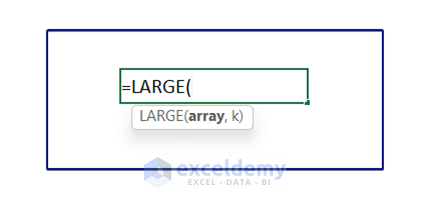
Arguments Explanation
| ARGUMENT | REQUIREMENT/OPTIONAL | DESCRIPTION |
|---|---|---|
| array | Required | The array from which we need to find the Kth largest value |
| k | Required | An integer that indicates the position from the largest value, as the Nth position |
Version
- The LARGE function is available from Microsoft Office 2007.
- Here, we will use Microsoft Office 365.
Read More: How to Use VBA Large Function in Excel
How to Use Excel Large Function in Multiple Ranges: 2 Example
We have shown 2 examples where we used the LARGE function in multiple ranges. Like, in the first example, we will use the LARGE function to get the highest value for section A. Then, for the second example, we will combine the LARGE function with other functions such as INDEX and MATCH functions. By merging other functions with the LARGE function, we can solve different types of problems more efficiently.
Example 1: Using LARGE Function to Find the Highest Value from Multiple Ranges
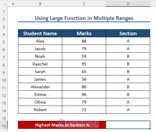
Here we have a dataset that represents the marks of two sections (Section A and Section B) of class 6. If we want to find the highest marks in Section A, we have to apply the formula for multiple ranges.
Steps:
- Write down the formula in cell D5. You must select the ranges among which you want the largest marks. In this case, we have selected the ranges of section A only.
=LARGE((C5:C6,C10,C13:C14),1)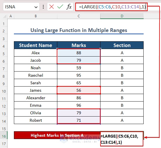
- Press ENTER to see the result.
- You will get the highest mark in section A, which is 88.

Formula Breakdown
- LARGE((C5:C6,C10,C12:C13),1): Here, among array (C5:C6,C10,C12:C13) the LARGE function finds the highest value (K=1).
Read More: How to Find Largest Number in Excel
Example 2: Merging INDEX, MATCH, and LARGE Functions to Get the Nth Largest Values
If we want to know the top 3 scores with the student’s name, we can merge the INDEX, MATCH, and LARGE functions.
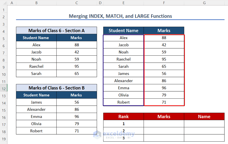
Steps:
- Write the formula in cell F17.
=INDEX($F$5:$F$14,MATCH(LARGE($F$5:$F$14,$E17),$F$5:$F$14,0))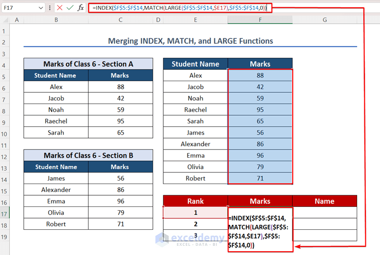
- Now, hit the ENTER key.
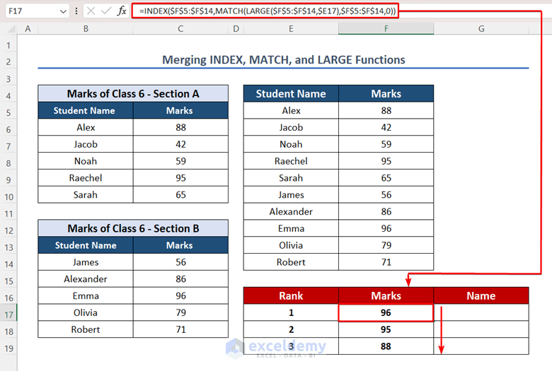
- Here we have the highest mark 96 as a result.

- Copy it down to cell F19.
- Thus, we have determined the top three marks.
Formula Breakdown
- LARGE($F$5:$F$14,$E17): This portion finds the highest marks (E17= 1) in the range F5:F14.
- MATCH(LARGE($F$5:$F$14,$E17),$F$5:$F$14,0): Afterward, this portion provides the row number of the top scorer in the range F5:F14.
- INDEX($F$5:$F$14,MATCH(LARGE($F$5:$F$14,$E17),$F$5:$F$14,0)): Finally, the INDEX function will return the marks from range F5:F14.
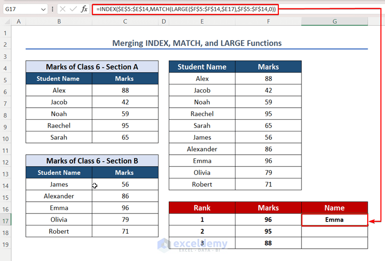
- To get the student’s name, enter the formula in cell G17.
=INDEX($E$5:$E$14,MATCH(LARGE($F$5:$F$14,$E17),$F$5:$F$14,0))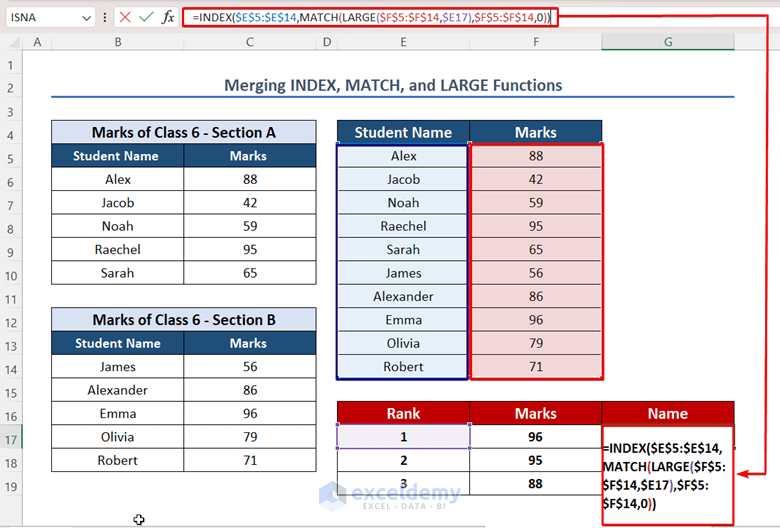
- After that, click ENTER.
- We will get the name of the top scorer.
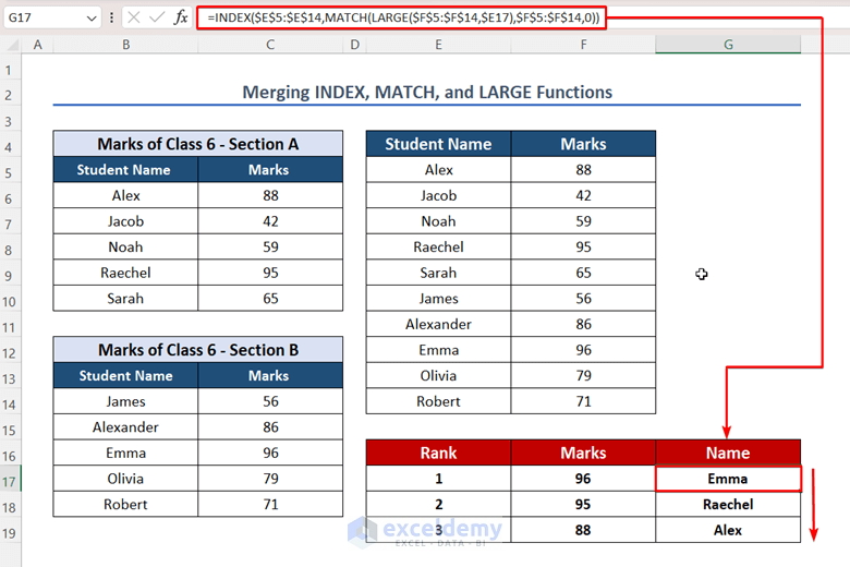
- Copy the formula down to cell G19.
- We will find the names of the top three scorers.
Formula Breakdown
- LARGE($F$5:$F$14,$E17): This portion finds the highest marks (E17= 1) in the range F5:F14.
- MATCH(LARGE($F$5:$F$14,$E17),$F$5:$F$14,0): Then, this portion provides the row number of the top scorer in the range F5:F14.
- INDEX($E$5:$E$14,MATCH(LARGE($F$5:$F$14,$E17),$F$5:$F$14,0)): Lastly, the INDEX function will return the associated data with the highest value from the range F5:F14.
Read More: How to Use Excel LARGE Function with Criteria
Download Practice Workbook
You may download the following Excel workbook for better understanding and practice it by yourself.
Conclusion
In these two examples, I have shown multiple criteria for using the Excel LARGE function in multiple ranges. There may be some different situations where the formula needs to be modified. If you have any questions regarding this topic, please comment so that we can help.
Related Articles
- How to Use Excel LARGE Function with Text
- How to Use Excel LARGE Function with Duplicates in Excel
- How to Use LARGE Function with VLOOKUP Function in Excel
- How to Lookup Next Largest Value in Excel
- How to Find Second Largest Value with Criteria In Excel
- How to Use LARGE and SMALL Function in Excel
<< Go Back to Excel LARGE Function | Excel Functions | Learn Excel

