Method 1 – Nesting LARGE, COUNTIF, MAX, MIN, INDIRECT, and ROW Functions to Find the N-th Largest Value from Data That Contains Duplicates
Steps:
- Use this formula in cell H5.
=LARGE(IF(COUNTIF(E$5:E$12,ROW(INDIRECT(MIN(E$5:E$12)&":"&MAX(E$5:E$12)))),ROW(INDIRECT(MIN(E$5:E$12)&":"&MAX(E$5:E$12)))),G5)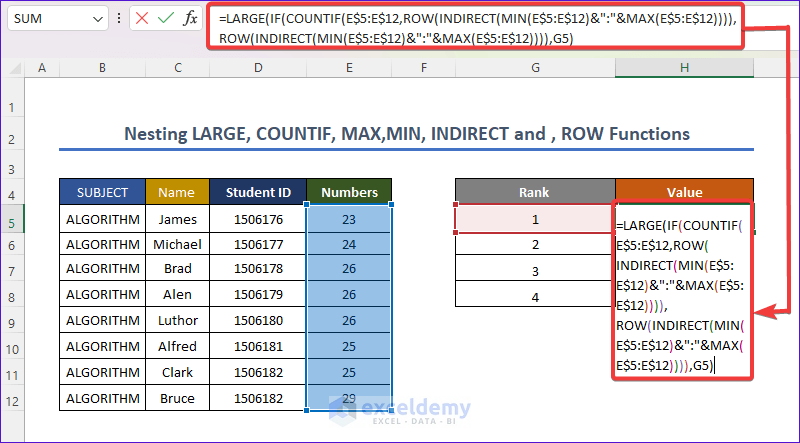
- Press ENTER.
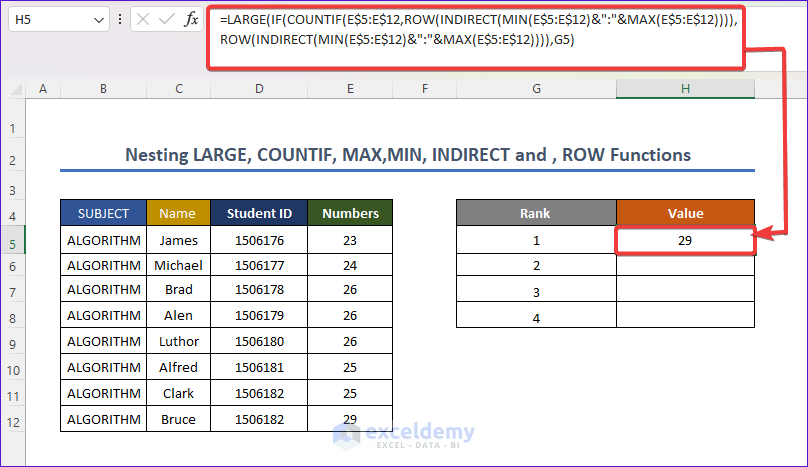
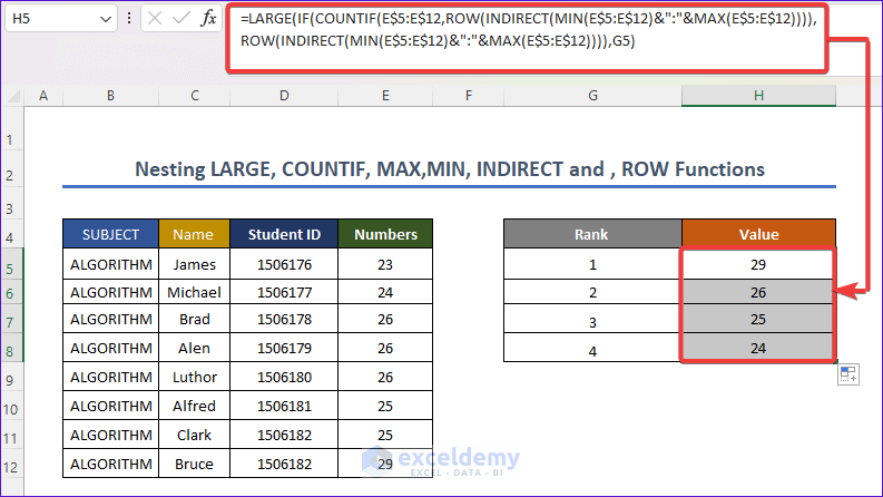
- Use the AutoFill tool to copy the formula.
Formula Breakdown
- ROW(INDIRECT(MIN(E$5:E$12)&”:”&MAX(E$5:E$12) gives the row reference of maximum value to the minimum value of the array and the INDIRECT function gives the reference.
- COUNTIF(E$5:E$12,ROW(INDIRECT(MIN(E$5:E$12)&”:”&MAX(E$5:E$12)))) counts how many numbers are duplicates.
- IF(COUNTIF(E$5:E$12,ROW(INDIRECT(MIN(E$5:E$12)&”:”&MAX(E$5:E$12)))),ROW(INDIRECT(MIN(E$5:E$12)&”:”&MAX(E$5:E$12)))),G5: the IF function returns the corresponding value highest to lowest without duplicates.
- =LARGE(IF(COUNTIF(E$5:E$12,ROW(INDIRECT(MIN(E$5:E$12)&”:”&MAX(E$5:E$12)))),ROW(INDIRECT(MIN(E$5:E$12)&”:”&MAX(E$5:E$12)))),G5) gives the large value corresponding to cell G5.
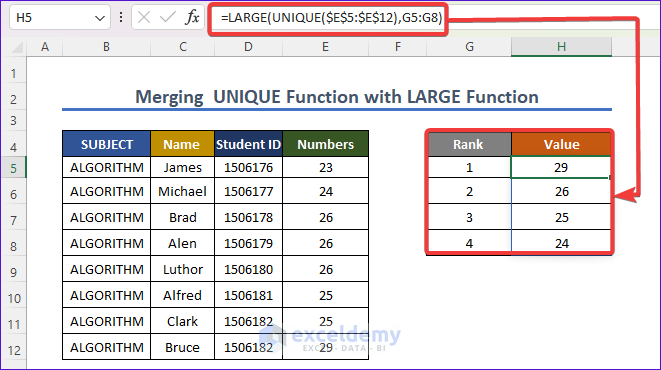
Method 2 – Merging UNIQUE and LARGE Functions to Find the Unique Largest Value
Steps:
- Use this formula in cell H5.
=LARGE(UNIQUE($E$5:$E$12),G5:G8)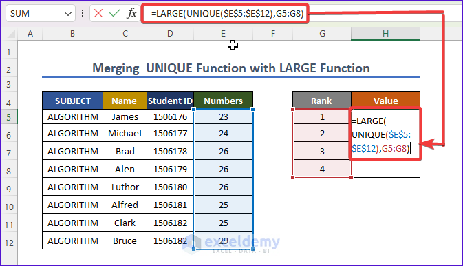
- Press ENTER.
Formula Breakdown
- UNIQUE($E$5:$E$12) finds out the unique value from selected cells of column E.
- =LARGE(UNIQUE($E$5:$E$12),G5:G8) returns the large function in column G.
Method 3 – Using IFERROR, FREQUENCY, MATCH, and ROW in the LARGE Function to Find Unique Largest Value
Steps:
- Use this formula in cell H5.
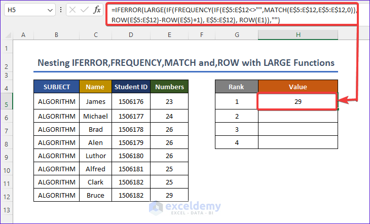
=IFERROR(LARGE(IF(FREQUENCY(IF(E$5:E$12<>"",MATCH(E$5:E$12,E$5:E$12,0)),ROW(E$5:E$12)-ROW(E$5)+1), E$5:E$12), ROW(E1)),"")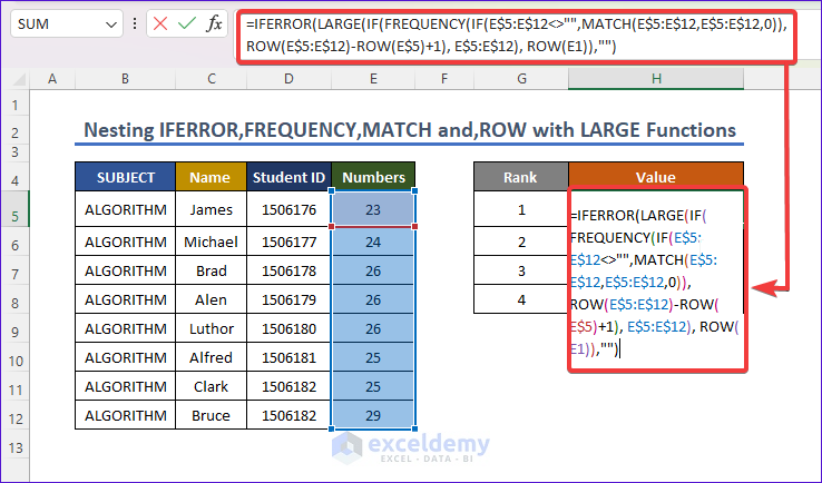
- Click ENTER.
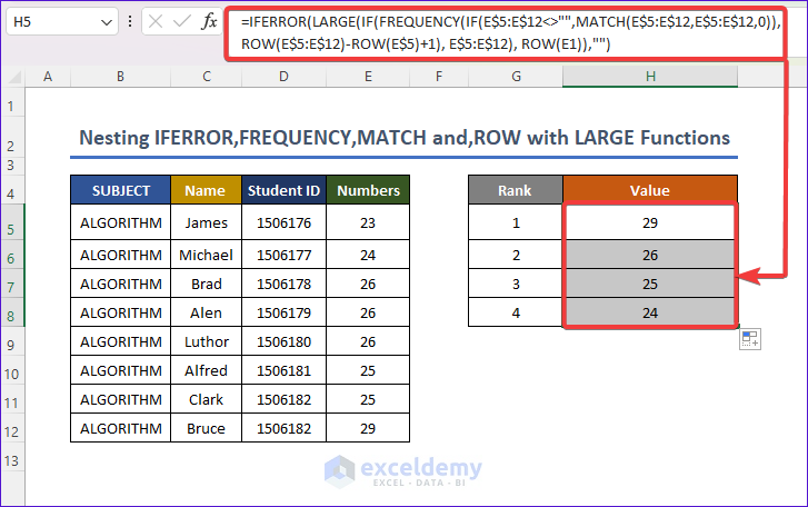
- Apply the AutoFill tool to get the final result.
Formula Breakdown
- IF(E$5:E$12<>””,MATCH(E$5:E$12,E$5:E$12,0)) in this formula the MATCH function finds out the corresponding relative position when they do not find the relative duplicate value. If they find a duplicate, the number indicating the relative position will be identical.
- FREQUENCY(IF(E$5:E$12<>””,MATCH(E$5:E$12,E$5:E$12,0)),ROW(E$5:E$12)-ROW(E$5)+1), E$5:E$12) frequency returns how many times same values are repeated and makes the corresponding position value become zero after first one occurs.
- IF(FREQUENCY(IF(E$5:E$12<>””,MATCH(E$5:E$12,E$5:E$12,0)),ROW(E$5:E$12)-ROW(E$5)+1), E$5:E$12), ROW(E1)) we find the sorted value lowest to highest and the position of repeated value becomes false.
- LARGE(IF(FREQUENCY(IF(E$5:E$12<>””,MATCH(E$5:E$12,E$5:E$12,0)),ROW(E$5:E$12)-ROW(E$5)+1), E$5:E$12), ROW(E1) gives the sorted value of lowest to highest.
- IFERROR(LARGE(IF(FREQUENCY(IF(E$5:E$12<>””,MATCH(E$5:E$12,E$5:E$12,0)),ROW(E$5:E$12)-ROW(E$5)+1), E$5:E$12), ROW(E1)),””) the IFERROR function gives an error if an error is found. Here no error is found.
Download the Practice Workbook
You may download the following workbook to practice yourself.
Related Articles
- How to Use Excel LARGE Function with Criteria
- How to Use Excel LARGE Function in Multiple Ranges
- How to Use Excel Large Function with Text
- How to Find Second Largest Value with Criteria In Excel
- How to Use LARGE and SMALL Function in Excel
- How to Use LARGE Function with VLOOKUP Function in Excel
<< Go Back to Excel LARGE Function | Excel Functions | Learn Excel

