In this article, we will demonstrate how to use the LARGE function with criteria in Excel.
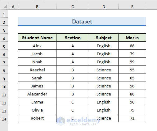
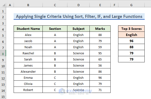
Using the following dataset containing the marks in Science and English of 2 sections of a class (Section A and Section B), let’s work through some examples of finding the largest (or nth largest) values using the LARGE function with criteria.
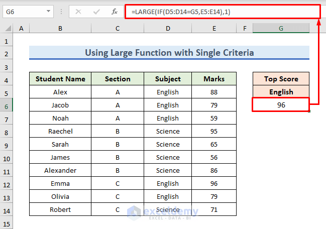
Example 1 – Using the LARGE Function with a Single Criterion
We can combine the IF function with the LARGE function to find the maximum value with a single criterion. Let’s find the highest mark in English from the combined dataset of sections A and B.
Steps:
- Enter the following formula in cell G6:
=LARGE(IF(D5:D14=G5,E5:E14),1)- Press Enter to return the result.
The highest mark in English is 96, which is correct.
Example 2 – Using the LARGE Function with Multiple Criteria
We can apply multiple criteria in the LARGE function using OR / AND logic.
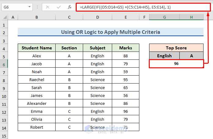
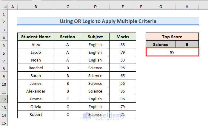
2.1 – Using OR Logic to Insert Multiple Criteria
Let’s find the highest mark in English or section A.
STEPS:
- Enter the following formula in cell G7:
=LARGE(IF((D5:D14=G5) +(C5:C14=H5), E5:E14), 1)- Press Enter to return the result.
In the dataset, the highest mark in English is 96 and in section A it is 88. As 96 is greater than 88, the result is 96.
To find out the highest mark in Science or Section B:
- Enter Science and B in cells G5 and H5 respectively.
- Press Enter.
The result is 95, which is correct.
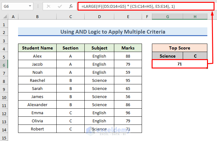
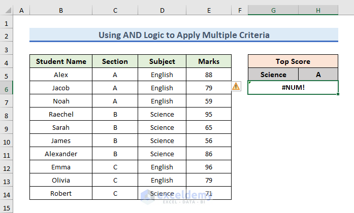
2.2 – Using AND Logic to Insert Multiple Criteria
To find the highest mark among the students of section C in Science, we’ll use AND logic.
Steps:
- Enter the following formula in cell G7:
=LARGE(IF((D5:D14=G5) * (C5:C14=H5), E5:E14), 1)- Press Enter to return the result.
71 is returned, which is correct.
Although the highest mark in Science is 95, it is in section B. In section C, the highest mark in Science is 71.

To find the top score in Science within section A:
- Type A in cell H5.
- Press Enter to proceed.
An error is returned, because there is no Science result in section A.
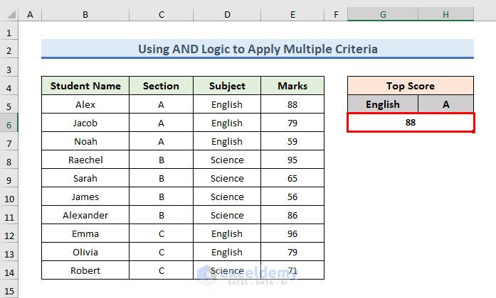
To find the top score in English within section A:
- Type English in cell G5.
- Press Enter to proceed.
The result is 88.
Read More: How to Use Excel LARGE Function in Multiple Ranges
Example 3 – Filter the Top n Values Using the LARGE Function with Criteria
We can easily filter the top n values based on both single and multiple criteria with the LARGE function.
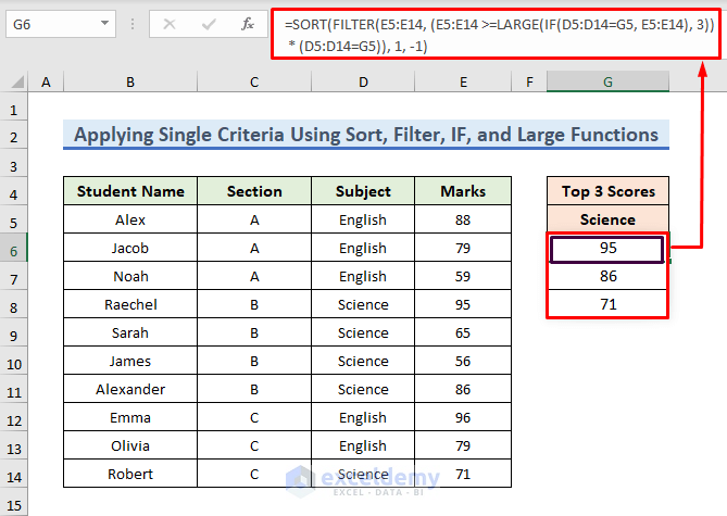
3.1 – Applying a Single Criterion Using the SORT, FILTER, IF, and LARGE Functions
Let’s filter out the top 3 marks based on a single criterion, for example, in Science.
.Steps:
- Enter the following formula in cell G6:
=SORT(FILTER(E5:E14, (E5:E14 >=LARGE(IF(D5:D14=G5, E5:E14), 2))- Press Enter to return the top 3 marks in Science.
To find the top 3 scores in English:
- Type English in cell G5.
- Press Enter.
The top 3 marks in English are returned. As 79 has come up twice, the result contains two 79s.
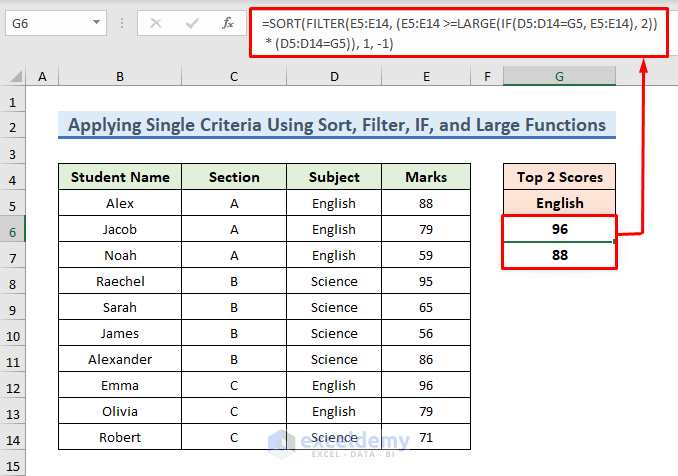
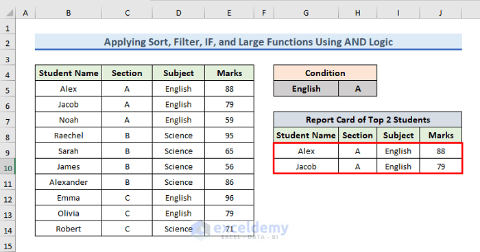
To find the top 2 scores in English, just replace 3 with 2 in the previous formula.
- So, the formula will be:
=SORT(FILTER(E5:E14, (E5:E14 >=LARGE(IF(D5:D14=G5, E5:E14), 2)) * (D5:D14=G5)), 1, -1)- Press Enter to return the top 2 marks in English.
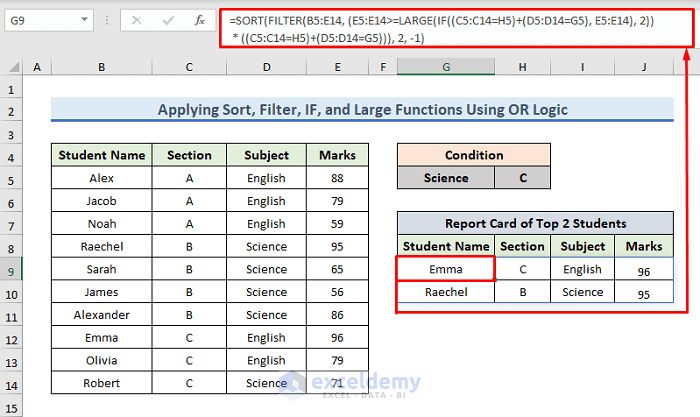
3.2 – Using the SORT, FILTER, IF, and LARGE Functions to Combine Criteria Using OR Logic
Here, we will extract the information of the top n values from the dataset if any one of multiple criteria is fulfilled.
Let’s find the top 2 scores in Section C or in Science.
Steps:
- Enter the following formula in cell G6:
=SORT(FILTER(B5:E14, (E5:E14>=LARGE(IF((C5:C14=H5)+(D5:D14=G5), E5:E14), 2))* ((C5:C14=H5)+(D5:D14=G5))), 2, -1)- Press Enter to return the top 2 marks in Section C or Science.
1st is Emma, where the condition of Section C is met.
2nd is Raechel, where the condition of Science is met.
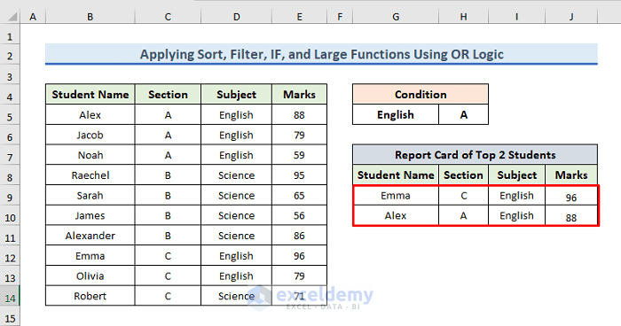
Similarly, we could find, say, the top 2 scores of section A or English.
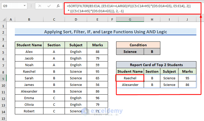
3.3 – Using the SORT, FILTER, IF, and LARGE Functions to Combine Criteria Using AND Logic
Now we’ll extract the information of the top n values from the dataset if both criteria are fulfilled. Let’s find the top 3 scores in section C in the subject Science.
Steps:
- Enter the following formula in cell G6:
=SORT(FILTER(B5:E14, (E5:E14>=LARGE(IF((C5:C14=H5)*(D5:D14=G5), E5:E14), 2)) * ((C5:C14=H5)*(D5:D14=G5))), 2, -1)- Press Enter to return the top 2 scores in Section C in Science.
Similarly, we can find, say, the top 2 scores in Section A in English.
Read More: How to Use Excel LARGE Function with Duplicates in Excel
Example 4 – Filtering the nth Largest Value Using the LARGE Function with Criteria
We can combine the IF and LARGE functions to determine the nth largest value using either a single or multiple criteria inside the LARGE function.
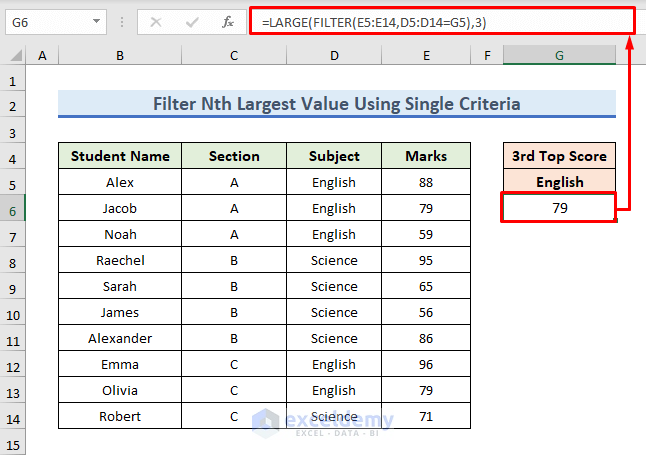
4.1 – Applying A Single Criterion to Find the nth Largest Value
Let’s find the 3rd highest mark in English from the combined dataset of sections A and B.
Steps:
- Enter the following formula in cell G6:
=LARGE(FILTER(E5:E14,D5:D14=G5),3)- Press Enter to return the result.
The 3rd highest mark in English is 79.
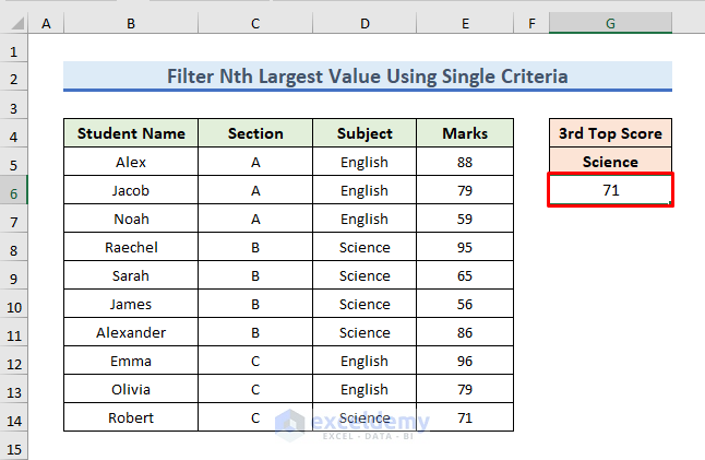
To find the 3rd largest mark in Science:
- Enter Science in cell G5 and press Enter.
The result is 71.
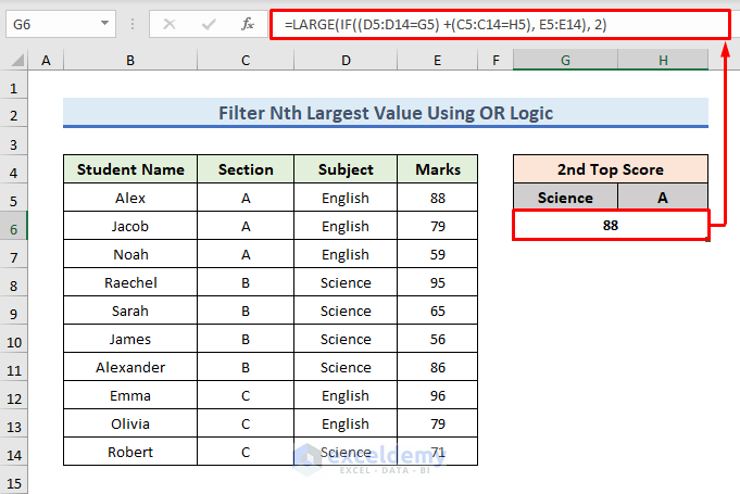
4.2 – Using OR Logic to Find the nth Largest Value
We’ll use OR logic to get the nth highest value from the dataset that meets one of multiple criteria.
Let’s find the 2nd highest mark of the combined dataset of Science and Section A.
Steps:
- Enter the following formula in cell G6:
=LARGE(IF((D5:D14=G5) +(C5:C14=H5), E5:E14), 2)- Press Enter to return the result.
The 2nd highest mark of the combined dataset of Science and section A is 88.
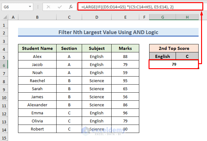
4.3 – Calculating the nth Largest Value Using AND Logic
We’ll use AND logic to get the nth highest value from the dataset that meets both both criteria.
Let’s find the 2nd highest mark in Section C for English.
Steps:
- Enter the following formula in cell G6:
=LARGE(IF((D5:D14=G5) *(C5:C14=H5), E5:E14), 2)- Press Enter to return the result.
The 2nd highest mark in Section C for Science is 79.
Read More: How to Find Second Largest Value with Criteria In Excel
Download Practice Workbook
To practice by yourself, download the following workbook.
Related Articles
- How to Use Excel Large Function with Text
- How to Lookup Next Largest Value in Excel
- How to Use LARGE Function with VLOOKUP Function in Excel
- How to Use LARGE and SMALL Function in Excel
<< Go Back to Excel LARGE Function | Excel Functions | Learn Excel

