Latest Posts From Bishawajit Chakraborty

We will demonstrate how to change table style by choosing table style, creating a custom table, resizing the table style, and removing table style. You will ...

Here's an example of a donut chart with multiple rings. Download the Practice Workbook Excel Doughnut Chart.xlsx What Exactly Is a ...
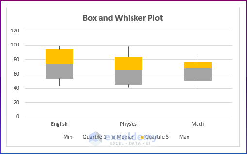
The box and whisker plot in Excel shows the distribution of quartiles, medians, and outliers in the assigned dataset. This article will demonstrate how to ...

In this article, you will learn how to - Merge IF, SEARCH, and ISNUMBER functions to add tags in Excel - Use the Excel Filter option to add tags in Excel ...

In this article, we will demonstrate how to: Apply a direct formula to calculate monthly payment. Use the PMT function to calculate monthly payment. ...

Here's an overview of where you can find the Accounting format to apply it to cells. Download the Practice Workbook Accounting Number ...

In this article, you will learn how to -Navigate within Excel cells and worksheets -Move across selected ranges for navigation -Use the scroll lock and ...

Rows in Excel provide a structured way for all the users to organize and reference data in an Excel worksheet. In this article, you will learn every detail ...

Excel theme refers to a predefined combination of colors, fonts, and effects that we can apply in our workbook to make it a consistent and professionally ...

Example 1 - Get the Array Dimensions with the Number of Elements in Excel Press F5 or click Run to run the VBA macro. Sub Array_Elements() Dim ...

One of the most frequent actions you complete each day while developing your reports, summary tables, dashboards, or even when using spreadsheets solely for ...
![[Fixed!] Excel Application-Defined or Object-Defined Error in VBA](https://www.exceldemy.com/wp-content/uploads/2023/05/4-Application-Defined-or-Object-Defined-Error-for-Name-Error-in-Excel-VBA.png?v=1697520112)
Reason 1 - Incorrect Worksheet Name Causes Application-Defined or Object-Defined Error in Excel VBA This happens when the name of the worksheet is already in ...
Method 1 - Activate Another Workbook by Workbook Name in Excel VBA This example will help you activate another workbook by closing your existing workbook when ...

Here is a sample video of our work on VBA LOOKUP values in a range in Excel. How to Open VBA Macro Editor in Excel VBA is a programming language ...

If you use Excel frequently, you are likely aware of how difficult it can be to handle. After you have more than a couple of worksheets, you need to manually ...
- 1
- 2
- 3
- …
- 7
- Next Page »
See Our Reviews at


Thank you so much Sharath for your response. If you have any questions, comments, or recommendations, kindly leave them in the comment section below.
Regards,
Bishawajit Chakraborty.
Hello Laura,
To save the file with the inserted images and send it via email, you can follow these steps:
Save the Workbook:
Attach the Workbook to Email:
Send the Email:
If you encounter any issues or have further questions, feel free to ask!
Thank you, Peter Abbott, for your wonderful question.
Here is the solution to your question:
This is the VBA code we have changed for multiple data columns and multiple timestamp columns.
First, input data for multiple columns, like below.
Now, paste the following in the module. Then, click on the Run button to see the output.
Finally, see the following output:
I hope this may solve your issue.
Bishawajit, on behalf of ExcelDemy
Thank you, DAWOOD, for your wonderful question.
In Excel, you can use a barcode font to create barcodes that include hyphens (“-“). Here are the steps to do it:
1. Download and Install a Barcode Font:
2. Enter Your Barcode Data:
I hope this may solve your issue. Also, please follow this article to get your answer with detailed explanations.
That’s it! You’ve created a barcode in Excel with hyphens included in the data. Remember that the actual appearance and functionality of the barcode depend on the specific barcode font you’re using, so make sure to choose a font that supports the format you need.
Bishawajit, on behalf of ExcelDemy
Thank you, ELEANOR TINDALL, for your wonderful question.
To apply multiple selections from a data validation list to specific columns (A and K) in an Excel sheet while restricting the rest of the columns to single-option entry, you can use VBA code. Here’s a modified version of the code that applies multiple selections only to columns A and K:
I hope this may solve your issue.
Bishawajit, on behalf of ExcelDemy
Thank you, STEVEN BRITTON, for your wonderful question.
Here is the explanation to your question.
It is true that the “Microsoft Date and Time Picker Control 6.0 (SP6)” is no longer available in Windows 11 and more recent versions of Microsoft Office. This control is no longer supported by Microsoft and is no longer included in the default ActiveX control set.
The most recent editions of Excel, including Windows 11, allow you to enter a date picker using a different method. You can now choose dates in Excel by using the built-in Microsoft “Calendar Control” date picker.
This article will help you how to add date and time picker control. Check this below link.
How to Use Excel UserForm as Date Picker
I hope this may solve your issue.
Bishawajit, on behalf of ExcelDemy
Thank you, KC, for your wonderful question.
Here is the explanation to your question.
It is true that the “Microsoft Date and Time Picker Control 6.0 (SP6)” is no longer available in Windows 11 and more recent versions of Microsoft Office. This control is no longer supported by Microsoft and is no longer included in the default ActiveX control set.
The most recent editions of Excel, including Windows 11, allow you to enter a date picker using a different method. You can now choose dates in Excel by using the built-in Microsoft “Calendar Control” date picker.
This article will help you how to add date and time picker control. Check this below link.
How to Use Excel UserForm as Date Picker
I hope this may solve your issue.
Bishawajit, on behalf of ExcelDemy
Thank you, KLAUDIUS, for your wonderful question.
Here is the solution to your question. Please take a look at the below steps.
I hope this may solve your issue.
Bishawajit, on behalf of ExcelDemy.
Thank you, FAJAR, for your wonderful question.
Here is the explanation to your question.
It is still possible for someone to obtain the cell value from another workbook without opening it using Excel VBA even if the source file is password- or other security-protected.
However, depending on the situation, accessing a protected file in this manner might be regarded as unethical or unlawful. It’s crucial to respect the security precautions taken by the file’s owner and to only access the data through legitimate, approved methods. Additionally, it is important to keep in mind that Excel offers a variety of protection options, and the efficacy of the protection depends on the particular technique used. While some security measures can be easily bypassed with a basic understanding of VBA, others are more robust and call for sophisticated techniques.
Because of this, it’s crucial to carefully examine the degree of protection needed for your unique use case and implement the proper security measures in accordance.
I hope this may solve your issue.
Bishawajit, on behalf of ExcelDemy
Thank you, RAFAL, for your wonderful question.
Here is the solution to your question.
This is the VBA code we have applied for multiple columns starting from row 2.
Now, for a better understanding of the output, you can see the below image.
I hope this may solve your issue.
Raiyan , on behalf of ExcelDemy
Thank you, Wlad, for your wonderful question.
Here is the explanation for your question.
Array Looping: The “For” loop iterates through the values in the “arr” array. The “LBound(arr, 1)” method returns the lower bound of the array’s first dimension, while the “UBound(arr, 1)” function delivers the upper bound of the array’s first dimension. The loop counter “i” takes values from the lower bound to the higher bound of the “arr” array’s first dimension.
Empty Loop: Because there are no statements or actions between the “For” and “Next” keywords, the loop looks to be an empty loop that does nothing significant.
I hope this may solve your issue.
Bishawajit, on behalf of ExcelDemy
Thank you, SAJAD, for your wonderful question.
Here is the solution to your question. Please take a look at the below steps.
I hope this may solve your issue.
Bishawajit, on behalf of ExcelDemy
Thank you, SIDDHARTH, for your wonderful question.
Here is the solution to your question. Please take a look at the below steps.
Here is our VBA code. Therefore, you can apply this code to solve your problem.
Here, you will see the final result in another sheet with names and marks.
I hope this may solve your issue.
Bishawajit, on behalf of ExcelDemy
Thank you, CHAD for your wonderful question.
Firstly, you cannot change the recipient’s name after emailing. When you apply the VBA code, the emails will pop up for sending. And on the Outlook email section, you can customize emails. So, you have to put the email address first in the recipient’s column.
This will do what you desire. If you have further queries, let us know.
Regards
Bishawajit, on behalf of ExcelDemy
Hi NICOLÁS,
Thanks for following our article. Please go through the whole article and create the template. And, you can use one ticker for only one sheet to import stock prices from any other website.
Let us know if your problem is fixed.
Regards,
Bishawajit Chakraborty
Author at ExcelDemy
Thank you JACK MACEY, for your wonderful question
If you want to import stock prices on a daily, weekly, monthly basis, you can visit this website link, from which we scraped our live data in accordance with this article.
Then, click on the Frequency option and select whatever you want for your desired frequency.
Finally, apply the rest procedures mentioned in the article. I hope this may solve your issue.
Bishawajit, on behalf of ExcelDemy
Thank you, MEREDITH, for your wonderful question.
Here is our modified VBA code. Therefore, you can apply this code to solve your problem but you can also modified this code for three digit numbers by using word “and” in our code section.
Here is the image of modified code where we have added the word “and”.
Here, you will see the final result.
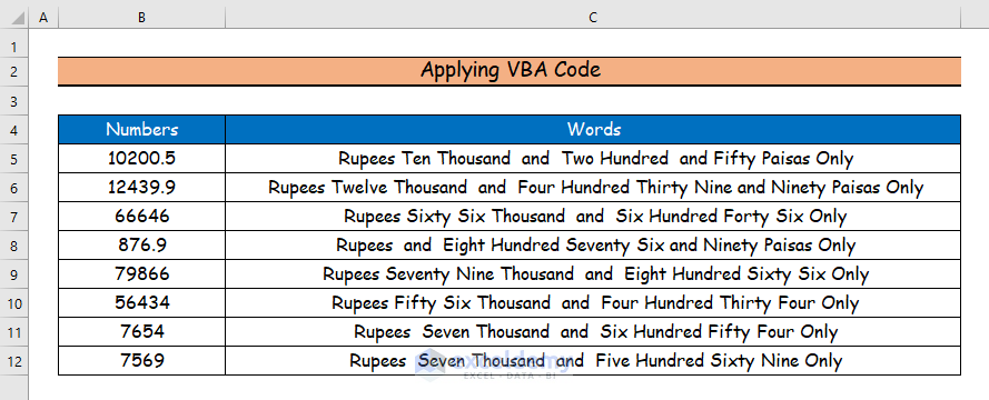
I hope this may solve your issue.
Bishawajit, on behalf of ExcelDemy
Thank you BRIAN for your wonderful question
If you want to import stock prices on a weekly basis, you can visit this website link, from which we scraped our live data in accordance with this article.
Then, click on the Frequency option and select Weekly for your desired frequency.
Finally, apply the rest procedures mentioned in the article. I hope this may solve your issue.
Bishawajit, on behalf of ExcelDemy
Thank you, Fred, for your wonderful question.
Firstly, go to the Home tab.
You can keep the decimal places of any number at any place by using the Increase Decimal and the Decrease Decimal icons here.
Bishawajit, on behalf of ExcelDemy
Thank you, SALWA for your wonderful question.
First off, you cannot change the time for a scheduled email; however, you can add the remaining date in the email using the VBA code. When you apply the VBA code, the emails will pop up for sending. And on the Outlook email section, you can customize emails with scheduled time
Then, using your Outlook account, you can set it up for a scheduled email. I hope this may solve your issue.
Bishawajit, on behalf of ExcelDemy
Thank you, JOHN SCURAS, for your comment.
You can use the below formula to determine your commission of the model.
=IF(H36>C33,SUMPRODUCT(–(H36>$C$33:$C$56),(H36-$C$33:$C$56),$D$33:$D$56)+C33*E33,C33*E33)
Here, H36 is the sales amount, C33 is your first Deal Size Range (High), C33:C56 is all values for Deal Size Range (High) column, D33:D56 is all values from the % incremental commission column, and E33 is the first value of the incremental commission (5%).
Best Regards,
Bishwajit
Team ExcelDemy
Thank you so much JOHN JOYCE for your comment. To set all the columns into text, you can follow the below steps accordingly.
After changing the format save the file and re-open it to check whether the data shows in the proper format.
Best Regards,
Bishwajit
Team ExcelDemy
Greetings AND74,
Thanks for noticing the error.
It will be OR(C5QUARTILE($C$5:$C$14,3)+1.5*$D$16) instead of OR(C5QUARTILE($C$5:$C$14,1)+1.5*$D$16).
We will make the corrections shortly.
Best Regards,
Bishwajit
Team ExcelDemy
Thank you, Edward Vinieratos, for your comment. According to your formula, your data seems quite large. It is hard to identify where the error lies. Can you please kindly share your excel file with us? We will create another Excel file with your desired result. We will reply to you back as soon as possible. Email Address: [email protected].
Thank you Edijs for your wonderful question. To edit the cell range follow these steps:
Firstly, enable the Microsoft Forms 2.0.
Secondly, type this code on to sheet 2.
Thirdly, type change the code from Module 1.
This should solve your problem. You can see the output from the following animated image.
If you have any further question, please let us know.
Regards
Bishawajit, on behalf of ExcelDemy
Thank you, Brian for the comment. You can use the following code to insert timestamp when value from a specific row change:
The following shows it working.
Now, for your second part of the comment. You can use this code for multiple rows:
The animated image shows it is working for two rows.
Regards
Bishawajit, on behalf of ExcelDemy
Thank you Prachi Davade for your wonderful question. You can change the
to
This will do what you desire. If you have further queries, let us know.
Regards
Bishawajit, on behalf of ExcelDemy
Thank you, Madan, for your comment. In our Excel file, this formula is working. Can you please share your excel file with us? Email Address: [email protected]. We will try to solve your problem as soon as possible.
Thank you so much, Peter, for your comment.
You will find your solution in the below steps. Please follow the steps accordingly.
Steps:

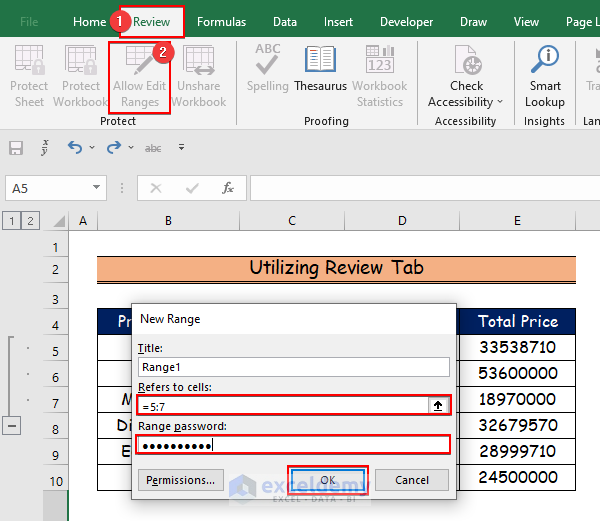
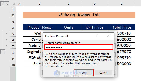
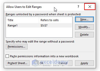
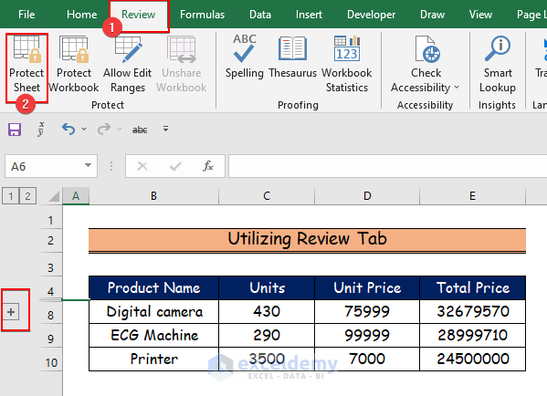
• Firstly, go to the Data tab.
• And, select the group option.
• Now, you will see here the plus (+) sign.
• Here, we have grouped the 5th, 6th, and 7th rows.
• Then, go to the Review tab.
• And, select the Allow Edit Ranges option.
• After that, choose the ranges.
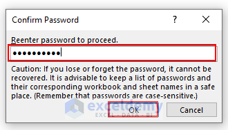
• And, type the password and click OK.
• Retype the password and click OK.
• Now remove this window.
• Firstly, go to the Review tab.
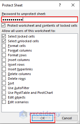
• Secondly, select the Protect Sheet option.
• Now, write your password.
• And, click OK.
• Then, retype your password and click OK.
• So, if you click on the plus (+) sign, it will show you the given result you want.
Hello Rash,
Thank you for your comment. If you want to send a table within the email body for any range, then you have to create a table in any worksheet. For this, you will follow our Method No.3 where we have used a VBA code to send an active sheet within the email body. Firstly, you can create a table in this active sheet and send this sheet with your table within the email body. Can you please share your Excel file with us? We will customize the file according to your requirements. Email address [email protected].
Regards,
Bishawajit Chakraborty (Exceldemy Team)
Thank you, Dhroov, for your comment. In our Excel file, this formula is working. Can you please share your excel file with us? Email Address: [email protected]. We will try to solve your problem as soon as possible.