Method 1 – Nesting the IF Function with Multiple Functions
- Open your Excel spreadsheet.
- In cell D5, enter the following formula:
=IF(ISNUMBER(SEARCH("@example.com",C5)),B5,"")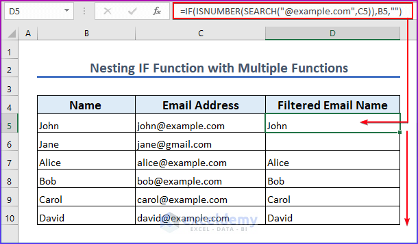
Formula Breakdown:
- The SEARCH function looks for the text string @example.com in cell C5. If found, it returns the position of the first character where @example.com appears. Otherwise, it returns an error.
- The ISNUMBER function checks if the SEARCH result is a number (indicating that @example.com was found in C5). If true, it returns TRUE; otherwise, FALSE.
- The IF function evaluates the ISNUMBER condition. If true, it returns the value in cell B5; otherwise, an empty string.
- Press Enter.
- To apply this formula to other cells, use the Fill Handle icon and drag it down from D5 to D10.
This technique extracts data from email addresses with the specified domain name. If @example.com appears in an email address in cell C5, the formula returns the corresponding value from cell B5. Otherwise, it returns an empty string.
Method 2 – Combining the TEXTJOIN Function with Multiple Functions
- In cell D5, enter the following formula:
=TEXTJOIN(", ",TRUE,IF(ISNUMBER(SEARCH("@example.com",C5:C10)),B5:B10,""))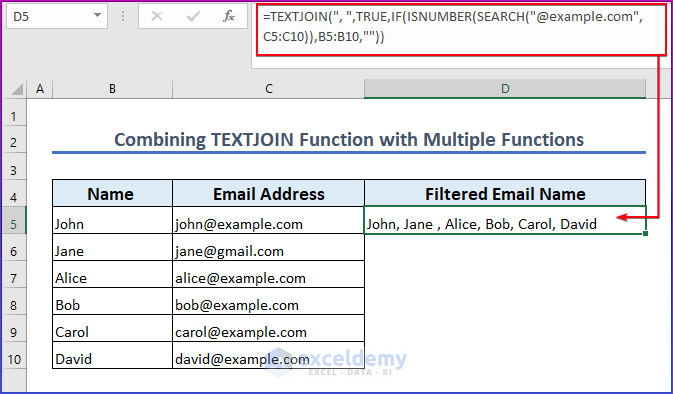
Formula Breakdown:
- The SEARCH function searches for @example.com in cells C5:C10. If found, it returns the position; otherwise, an error.
- The ISNUMBER function checks if the SEARCH result is a number (indicating @example.com was found). If true, it returns TRUE; otherwise, FALSE.
- The IF function evaluates each value in the range B5:B10. If the corresponding cell in C5:C10 contains @example.com, it returns the value; otherwise, an empty string.
- The TEXTJOIN function concatenates the matching values using a comma and space as delimiters (ignoring blanks).
- Press Enter to get the concatenated result in a single row.
Method 3 – Nesting the FILTER Function with Multiple Functions
- Open your Excel spreadsheet.
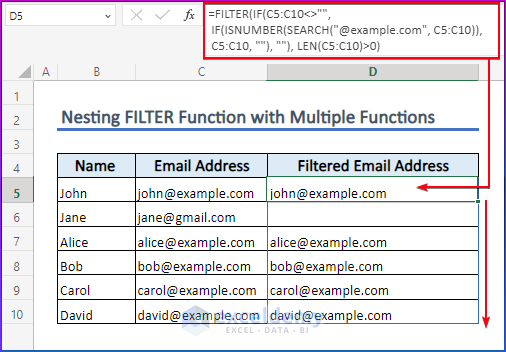
- In cell D5, enter the following formula:
=FILTER(IF(C5:C10<>"", IF(ISNUMBER(SEARCH("@example.com", C5:C10)), C5:C10, ""), ""), LEN(C5:C10) > 0)
Formula Breakdown:
- The SEARCH function checks if @example.com appears in each cell within the range C5:C10. If found, it returns the position; otherwise, an error.
- The ISNUMBER function determines if the SEARCH result is a number (indicating that “@example.com” was found). If true, it returns the corresponding value from C5:C10; otherwise, an empty string.
- The outer IF function evaluates whether each cell in C5:C10 is blank. If not blank, it passes the value to the inner IF function; otherwise, it returns an empty string.
- The FILTER function then filters the non-blank values, returning them as a vertical array.
- Press Enter.
- To apply this formula to other cells, use the Fill Handle icon and drag it down from D5 to D10.
Method 4 – Applying the Filter Command
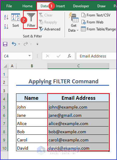
- Select the Email Address column in your Excel sheet.
- Click the Filter command from the Data tab. This applies a filter to the selected column.
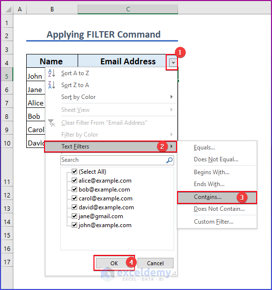
- You can filter email addresses based on your preferences. Click the drop-down arrow next to the email address column heading.
- Choose Text Filters and then select Contains.
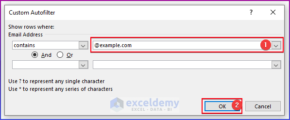
- Enter the domain @example.com in the text box.
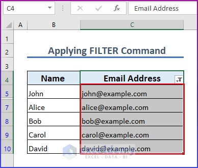
- Excel will filter and display only the email addresses containing the chosen domain.
- You’ll see the filtered results in the image below.
Method 5 – Using Data Validation to Filter Invalid Email Addresses
- Open your Excel spreadsheet.
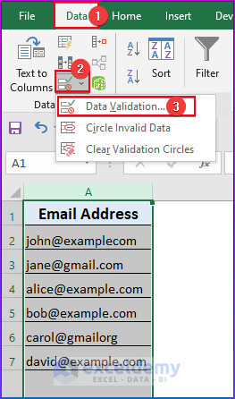
- Select the column containing email addresses (let’s assume it’s column A).
- Click on the Data tab.
- Choose Data Validation from the menu.
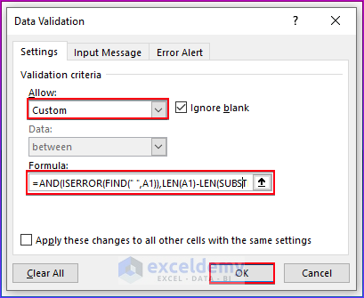
- In the Data Validation dialog box, select the Custom option.
- Enter the following formula in the Formula field:
=AND(ISERROR(FIND(" ",A1)),LEN(A1)-LEN(SUBSTITUTE(A1,"@",""))=1,IFERROR(SEARCH("@",A1)<SEARCH(".",A1,SEARCH("@",A1)),0),NOT(IFERROR(SEARCH("@",A1),0)=1),NOT(IFERROR(SEARCH(".",A1,SEARCH("@",A1))-SEARCH("@",A1),0)=1),LEFT(A1,1)<>".",RIGHT(A1,1)<>".")- This formula checks several conditions to determine if an email address is valid:
- It ensures there are no spaces in the address.
- It verifies that there is exactly one “@” symbol.
- It confirms that the “@” symbol appears before the “.” symbol.
- It checks that the address doesn’t start or end with a period.
- Click OK to apply the validation rule.
- Click the tiny triangle next to Data Validation again.
- Select Circle Invalid Data from the menu.
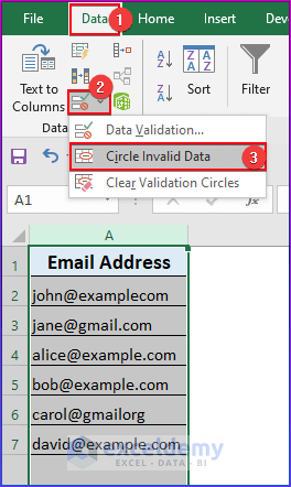
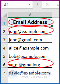
- You’ll notice that invalid email addresses are now highlighted with a red circle.
- By default, this operation starts from cell A1, so it will also encircle A1 if it contains an invalid email address.
Download Practice Workbook
You can download the practice workbook from here:
<< Go Back to Data | Filter in Excel | Learn Excel
Get FREE Advanced Excel Exercises with Solutions!
