How to Filter in Excel with Merged Cells (Step-by-Step Procedure)

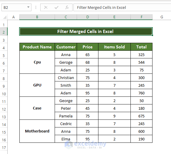
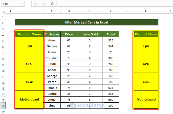
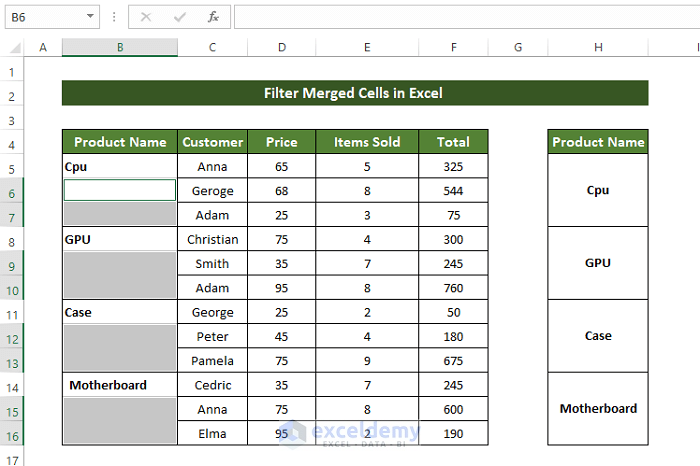
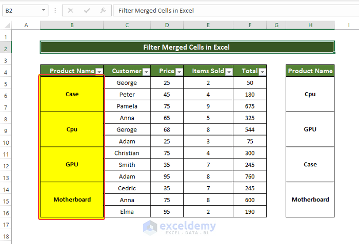
We will use a dataset of Product Names in merged cells to demonstrate how you can filter based on them.

Steps

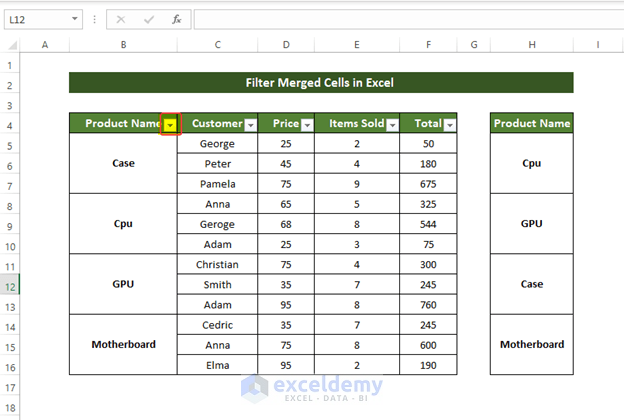
• Select the table and click the Filter icon from the Sort and Filter group in the Data tab.

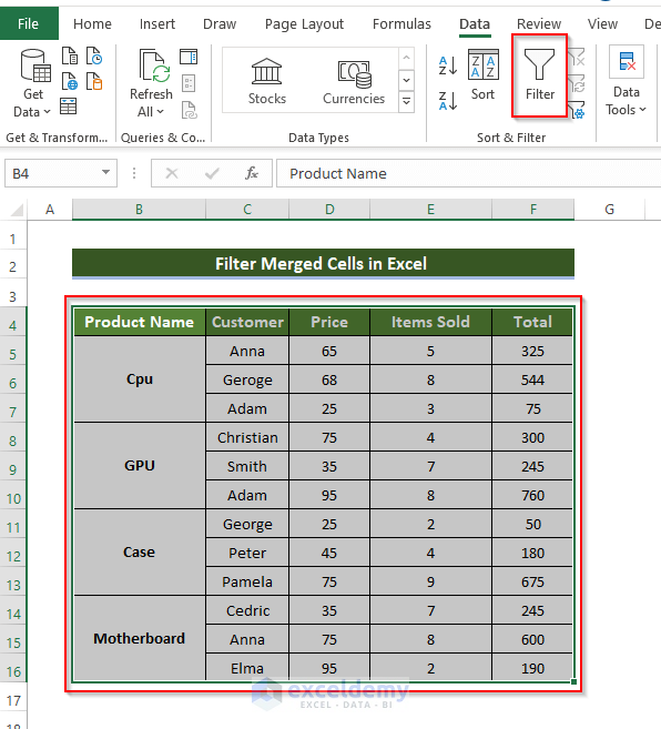
• After clicking the Filter icon, you will see drop-down icons in every header in the table.

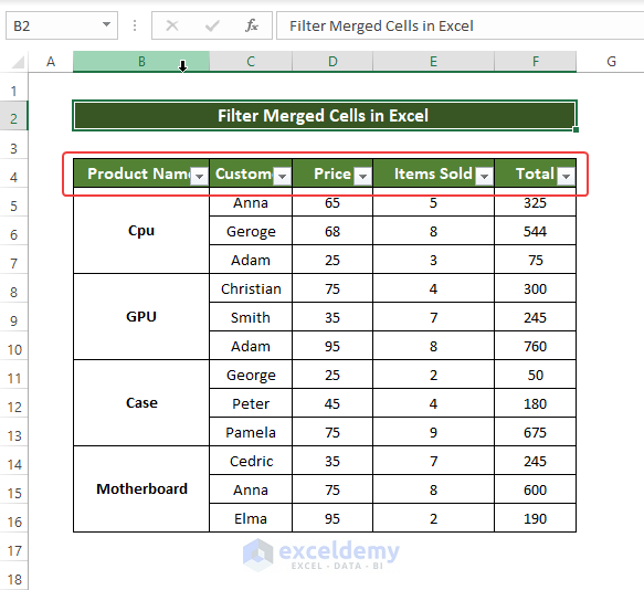
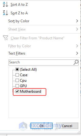
• We selected the drop-down icon of the Product Name column and selected only the motherboard option, then applied the filter with OK.

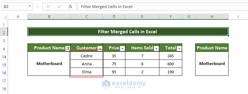
• Only one entry from cell C14 is showing instead of all three entries.

• Copy the product column’s entries to other cells for later use.

• Select the cell range of cells B5:B17 and, from the Home tab, go to Merge & Center.

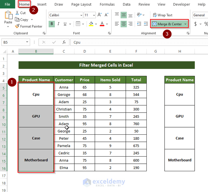
• All the cells in the Product Name will be unmerged. There will be empty cells in between the rows.
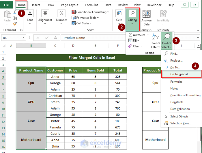
• Select the range of cells B5:B16.
• From the Home tab, go to Find and Select under Editing.
• After clicking Find and Select, a new dropdown menu will appear. From that menu, click Go To Special.

• A small window opens. Select Blanks and click on OK.

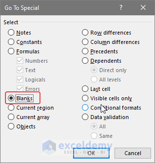
• All of the blank cells in the column Product Name are selected.

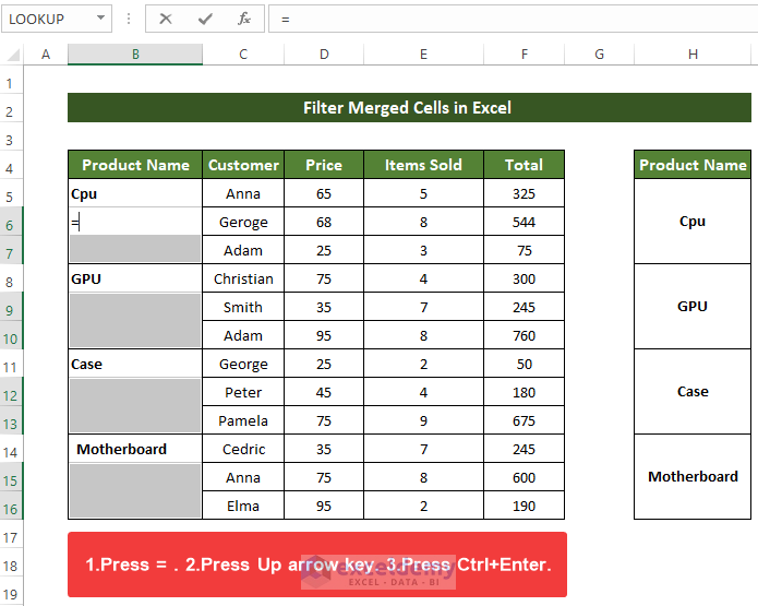
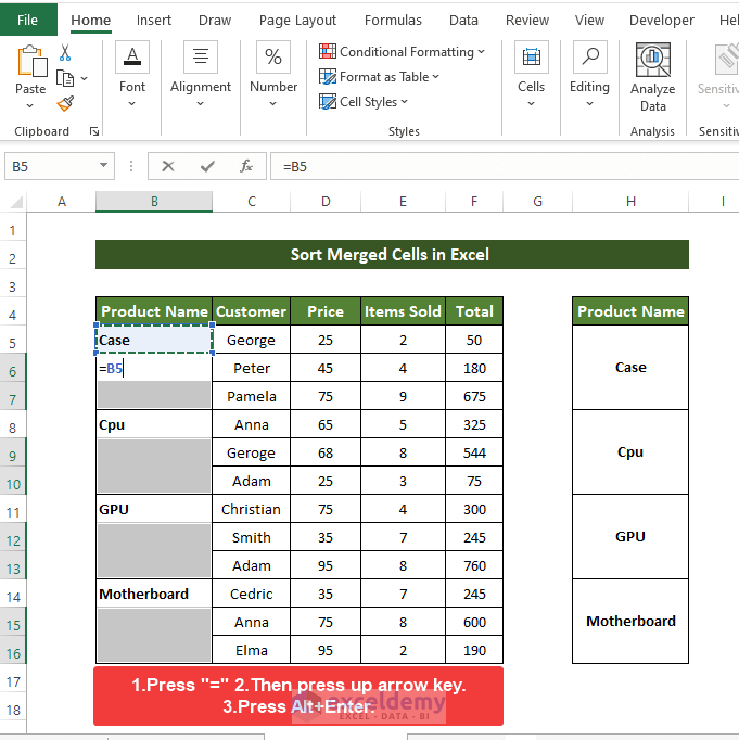
• Press “=”.
• Press up the arrow. 
• Press Alt + Enter.

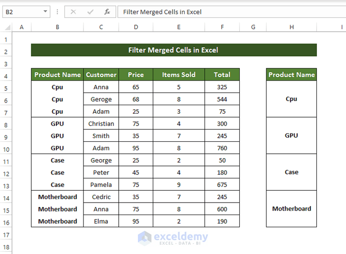
• All of the blank spaces will then be filled up by the value of the nearest neighbor above it.

• Select the range of cells H5:H16 and click Format Painter.
• Select the cells from B5:B16.

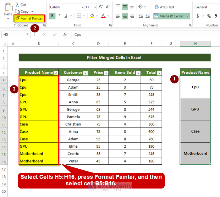
• It will turn all the cells into the same merged format as before.

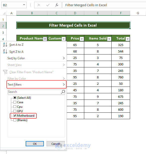
• Click the small drop-down menu on the corner of the Products Name

• From the dropdown filter menu, check Motherboard from Text Filter and then click OK.

• Unlike the first time, all available entries are visible. That means the filtering process was successful.

Read More: How to Filter Data in Excel using Formula

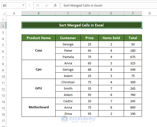
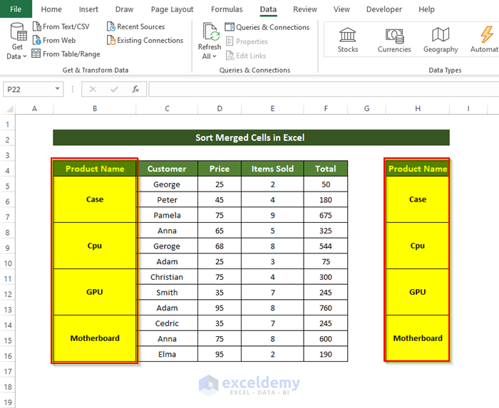
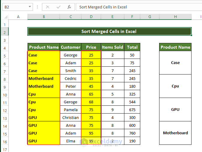
Sort Merged Cells in Excel

Steps

• The table shown below needs to be sorted, but there is a problem while sorting as text in column Product Name is in merged condition.

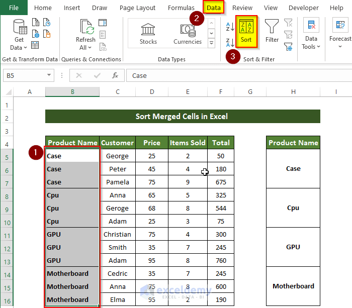
• Select the whole table and click the Sort icon from the Sort and Filter group in the Data tab.

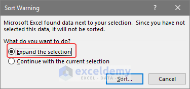
• Excel will ask whether you want to expand the selection. Select Expand the selection and click Sort.

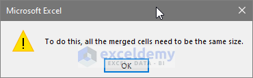
• There will be a small window saying that you need to have cells of the same size.

• Copy the product column’s entries to other cells for later use.

• Select the cell range B5:B17 then choose Merge & Center.

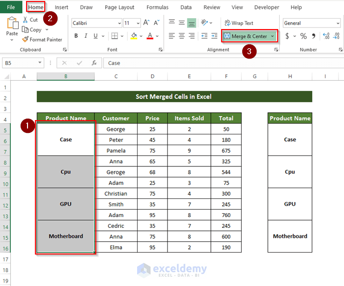
• All the cells in the Product Name will be unmerged. There will be empty cells in between the rows.
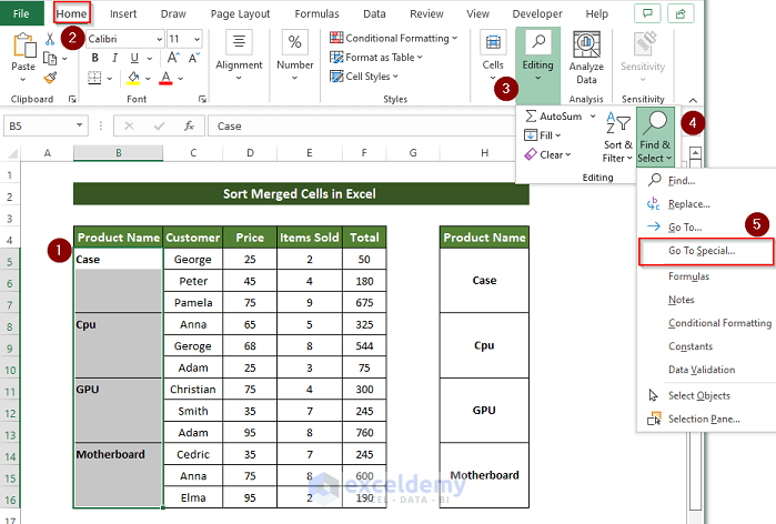
• Select the range of cells B5:B16 and, from the Home tab, go to Find and Select under Editing.
• Click Go To Special.

• A small window opens. Select Blanks and click OK.

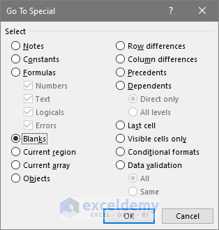
• All of the blank cells in the column Product Name are selected.
• Press “=”. Press the up arrow.
• Press Alt + Enter.

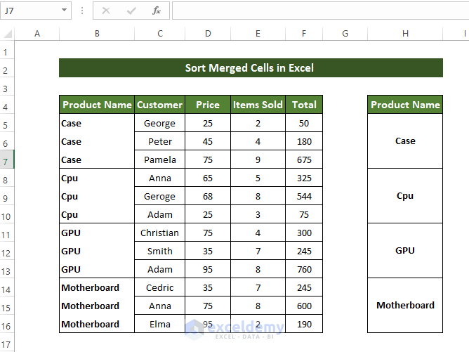
• All of the blank spaces will be filled up by the nearest neighbor above.

• Repeat the sorting process.

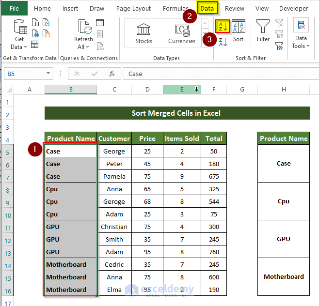
• You will get a notification saying whether you want to expand the selection. Select Expand the selection and click Sort.

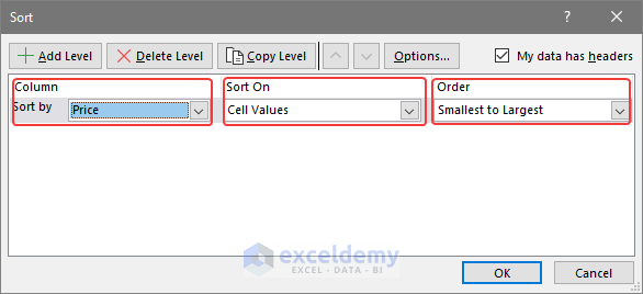
• Another new window appears asking to select the criteria Price in column sort by and in which cell the sorting going to apply on Sort On. Select the order Smallest to Largest in this case.

• You will see that the data is properly sorted.

Read More: How to Filter by List in Another Sheet in Excel

Download the Practice Workbook

<< Go Back to Data | Filter in Excel | Learn Excel