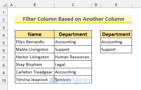
In this article, we’re going to show you 5 methods of how to use Excel to Filter a column based on another column. To demonstrate these methods, we’ve taken a dataset with 2 columns: “Name” and “Department”. Moreover, We’ll Filter based on the value of the “Department” column.
How to Filter Column Based on Another Column in Excel: 5 Ways
Method 1 – Using Advanced Filter to Filter Column Based on Another Column
Steps:
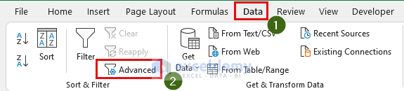
- From the Data tab, select Advanced. The Advanced Filter dialog box will appear.
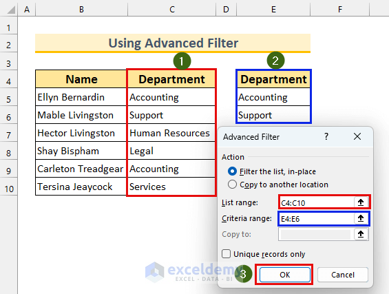
- Set the following cell ranges: C4:C10 as the List range, and E4:E6 as the Criteria range.
- Click on OK.
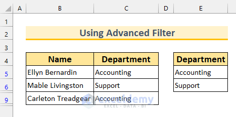
- The Name column is Filtered based on another column.
Method 2 – Filter a Column by Applying Excel COUNTIF Function
Steps:
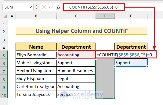
- Select the cell range D5:D10.
- Copy the following formula.
=COUNTIF($E$5:$E$6,C5)=0The COUNTIF formula is checking if the value from column C matches the value from column E. If the value is found, then 1 will be the output. Then, we’ll check if this value is 0. If yes, then we’ll get TRUE. Our Filtered column will continue the value FALSE.
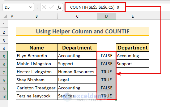
- Press Ctrl + Enter.
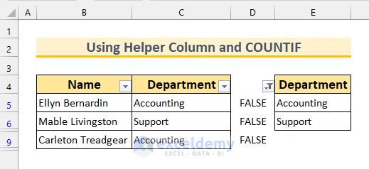
Here, we can see the matched values are showing FALSE.
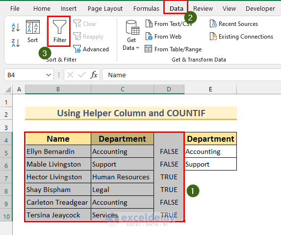
- Select the cell range B4:D10.
- From the Data tab, select Filter.
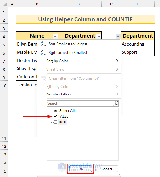
- Click on the Filter icon of column D.
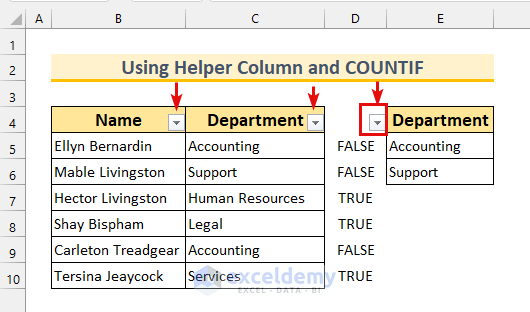
- Put a tick mark on FALSE.
- Press OK.
Thus, we’ve completed yet another method of Filtering columns based on another column.
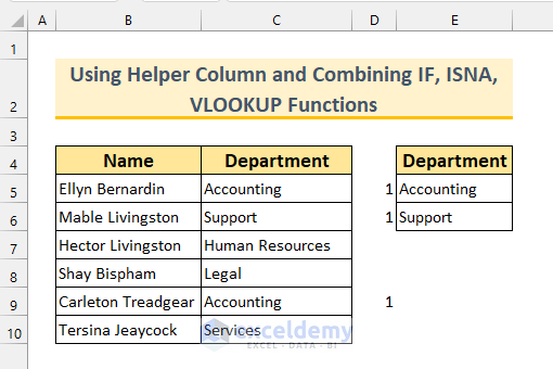
Method 3 – Combining IF, ISNA, VLOOKUP Functions in Excel to Filter Columns Based on Another Column
Steps:
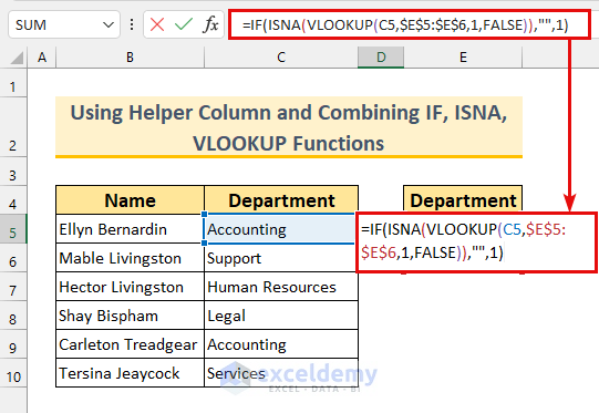
- Enter the following formula in cell D5:
=IF(ISNA(VLOOKUP(C5,$E$5:$E$6,1,FALSE)),"",1)Formula Breakdown
- VLOOKUP(C5,$E$5:$E$6,1,FALSE)
- Output: “Accounting”.
- The VLOOKUP function returns a value from an array or range. We’re looking for the value of “Accounting” in our array (E5:E6). There is only 1 column, hence we’ve put 1. Moreover, we’ve put FALSE for the exact match.
- Then our formula reduces to, IF(ISNA(“Accounting”),””,1)
- Output: 1.
- The ISNA function checks if a cell contains the “#N/A” error. If there is that error, then we’ll get TRUE as the output. Lastly, our IF function will work. If there is any error then we’ll get a blank cell, else we’ll get 1. As we found the value in our array, hence we’ve got the value 1 here.
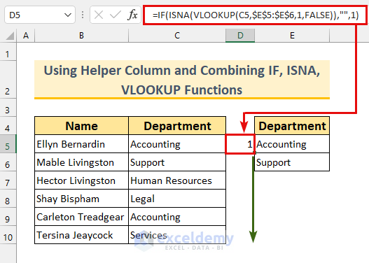
- Press Enter and AutoFill the formula.
We’ve received the value 1, as explained above.
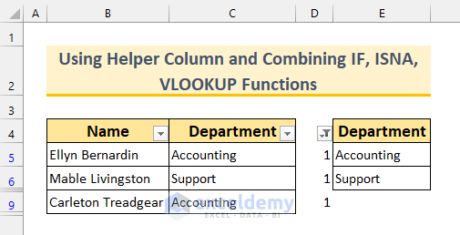
We can see there are 3 TRUE values.
- Following steps shown in method 2, filter the values containing 1 only.
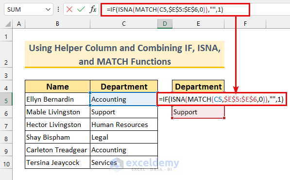
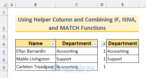
Method 4 – Incorporating IF, ISNA, MATCH Functions in Excel to Filter Column Based on Another Column
Steps:
- Copy the following formula in cell D5:
=IF(ISNA(MATCH(C5,$E$5:$E$6,0)),"",1)Formula Breakdown
- MATCH(C5,$E$5:$E$6,0)
- Output: 1.
- The MATCH function shows the position of a value in an array. Our lookup value is in cell C5. Our lookup array is in E5:E6, and we’re looking for the exact match, hence we put the 0.
- Then, our formula reduces to IF(ISNA(1),””,1)
- Output: 1.
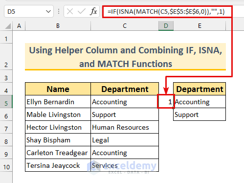
- The ISNA function checks if a cell contains the “#N/A” error. If there is that error, then we’ll get TRUE as the output. Lastly, our IF function will work. If there is any error then we’ll get a blank cell, else we’ll get 1. As we found the value in our array, hence we’ve got the value 1 here.
- Press Enter and AutoFill the formula.
We’ve got 1 as per the explanation above.
- Follow the steps shown in method 2 to filter the values containing 1 only.
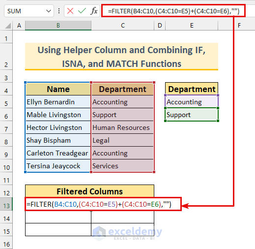
Method 5 – Filter Column Based on Another Column by Using FILTER Function in Excel
Available in Excel 2021 onward and Excel 365.
Steps:
- Copy the following formula in cell B13:
=FILTER(B4:C10,(C4:C10=E5)+(C4:C10=E6),"")Formula Breakdown
- Our array is B4:C10. We have two criteria that are connected with plus (+). That means if any of the criteria are fulfilled then we’ll get output.
- (C4:C10=E5)+(C4:C10=E6)
- Output: {0;1;1;0;0;1;0}.
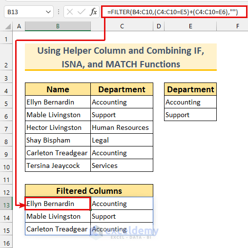
- We’re checking if the cell range contains our value from cells E5 and E6. Then, we got 3 values that meet our condition.
- We’re not defining any arguments in this formula.
- Press Enter.
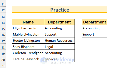
Practice Section
We’ve included practice datasets for each method in the Excel file.
Download Practice Workbook
<< Go Back to Data | Filter in Excel | Learn Excel
Get FREE Advanced Excel Exercises with Solutions!

Really good article! easily practice!
Hello Tony Jin,
You are most welcome. Your appreciation means a lot to us. You can explore more article related to these topic. Keep learning Excel with ExcelDemy.
Regards
ExcelDemy