How to Filter Multiple Columns Independently in Excel (5 Methods)

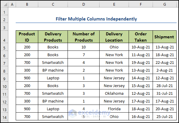
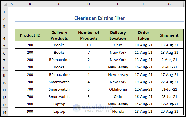
The dataset shows 10 delivery products of a company. It mentions the product ID, product name, quantity, delivery location, order date, and shipping date.

Method 1 – Filtering Data from Columns

Steps:

• Select the range of cells B4:G14.
• In the Home tab, click on the drop-down arrow of the Sort & Filter option and choose the Filter command from the Editing tab.

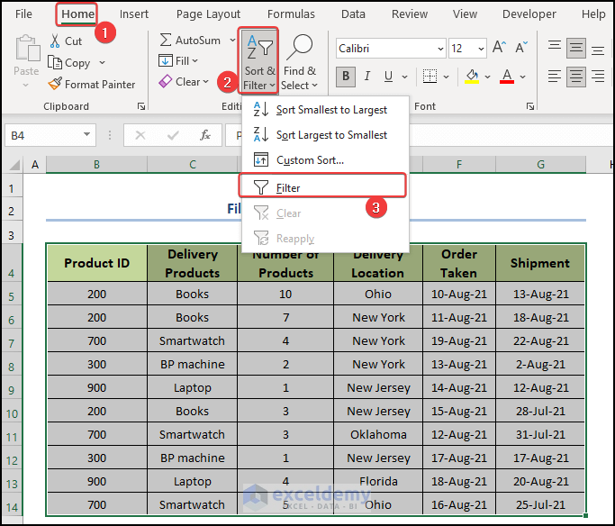
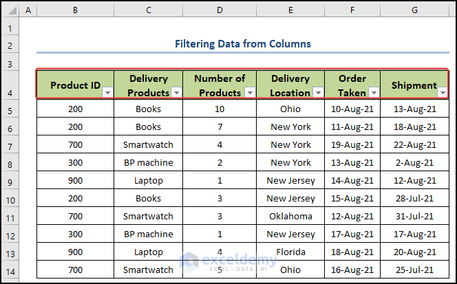
• A drop-down arrow will appear at the right-bottom corner of each column heading.

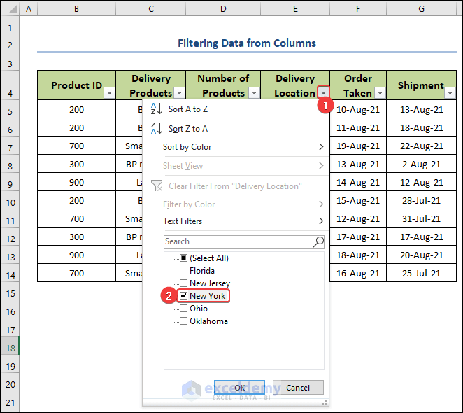
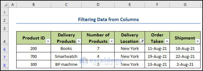
• Click on any drop-down arrow to apply the filter according to your desire. Here, we clicked on the drop-down arrow of the Delivery Location column and applied the filter only for New York.
• Click OK.

• You will see the result.

Read More: How to Filter Multiple Columns Simultaneously in Excel 

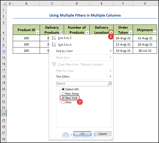
Method 2 – Using Multiple Filters in Multiple Columns

Steps:

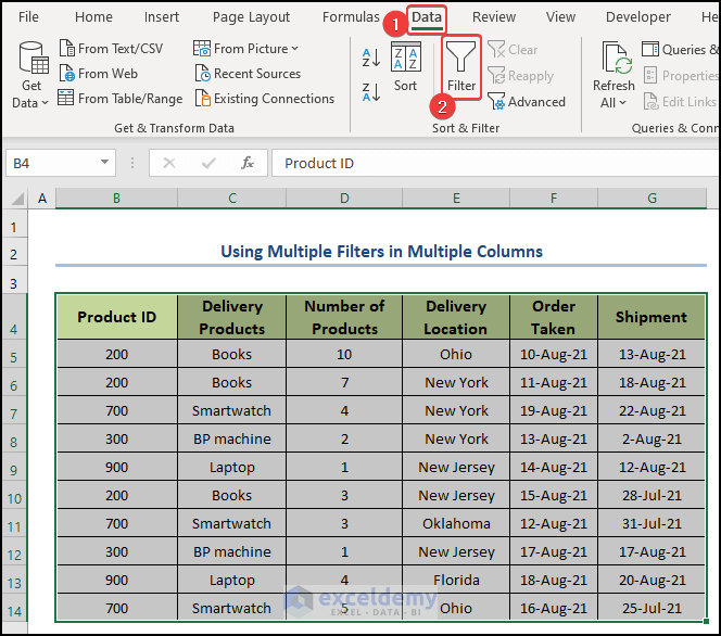
• Select the range of cells B4:G14.
• In the Data tab, click on the Filter option from the Sort & Filter group.

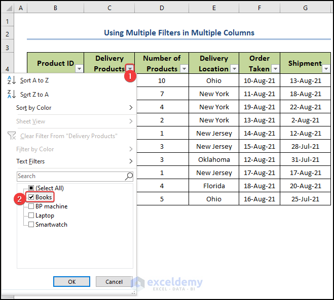
• A drop-down arrow will appear at the right-bottom corner of each column heading.
• Click on the drop-down arrow of the Delivery Product name and apply the filter for the Book product.
• Click OK.

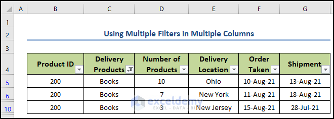
• All the book entities are filtered.

• For another filter, click on any drop-down arrow of another column according to your desire. Here, we clicked on the drop-down arrow of the Delivery Location column and applied the filter only for New York.
• Click OK.

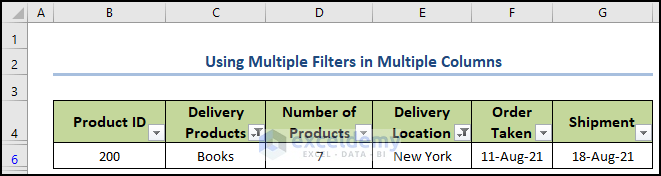
• You will see the result.

Read More: How to Hide Filter Buttons in Excel

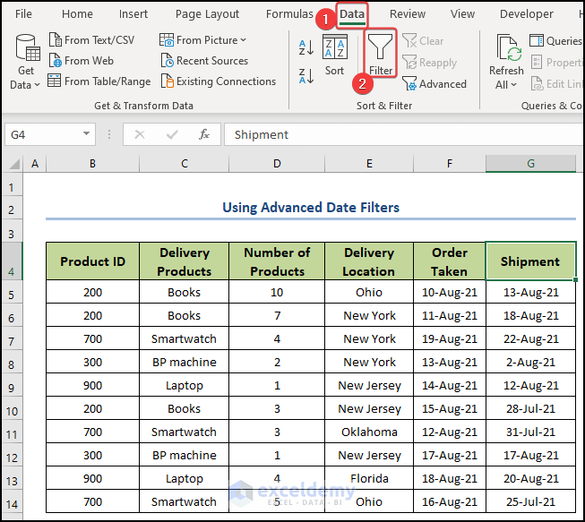
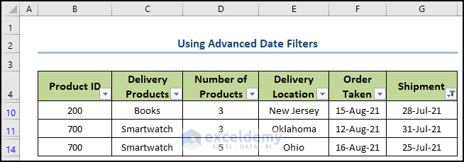
Method 3 – Using Advanced Date Filters

Steps:

• Select cell G4.
• In the Data tab, click on the Filter option from the Sort & Filter group.

• A drop-down arrow will appear at the right-bottom corner of each column heading.
• Click on the drop-down arrow of the Shipment column and check on the July option.
• Click OK.

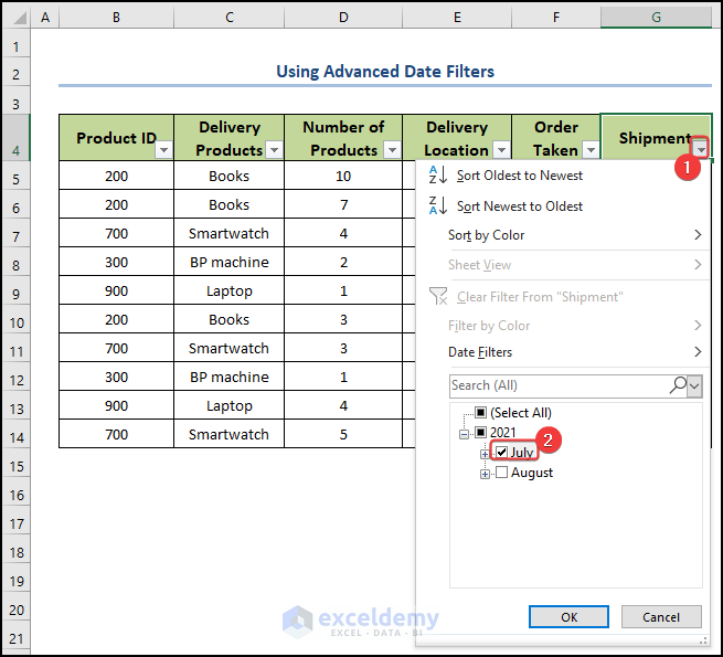
• The products to be delivered in July will be filtered.

Method 4 – Using Advanced Number Filters

Steps:

• Select cell B4:G4.
• In the Data tab, click on the Filter option from the Sort & Filter group.

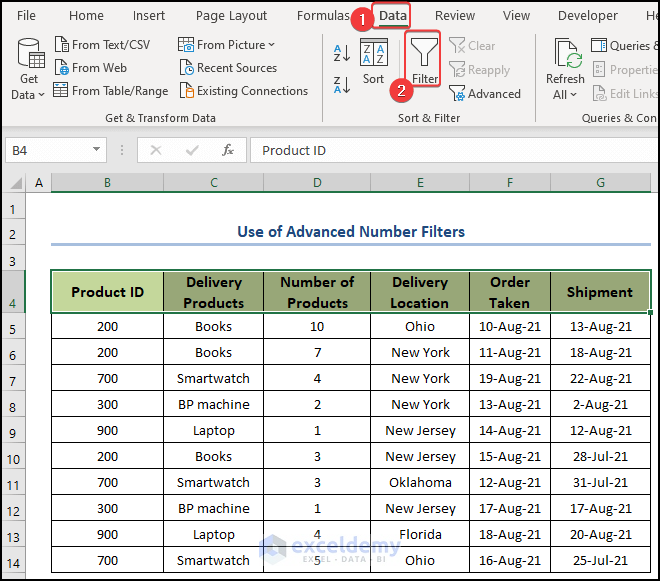
• A drop-down arrow will appear at the right-bottom corner of each column heading.
• Click on the drop-down arrow of the Product ID column and click on the Sort Smallest to Largest option.

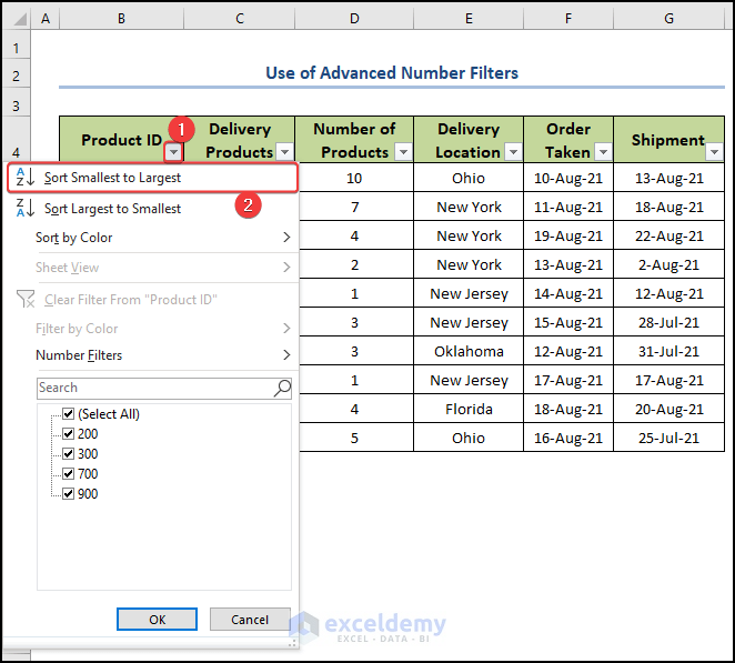
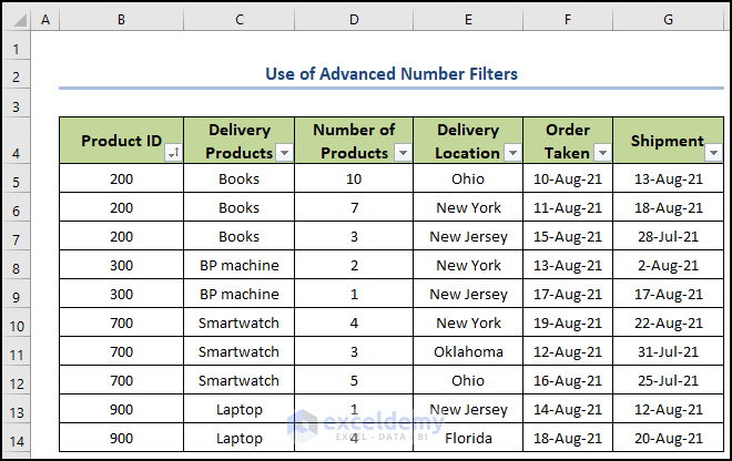
• The whole dataset will be sorted using the filter feature.

Read More: How to Filter Column Based on Another Column in Excel

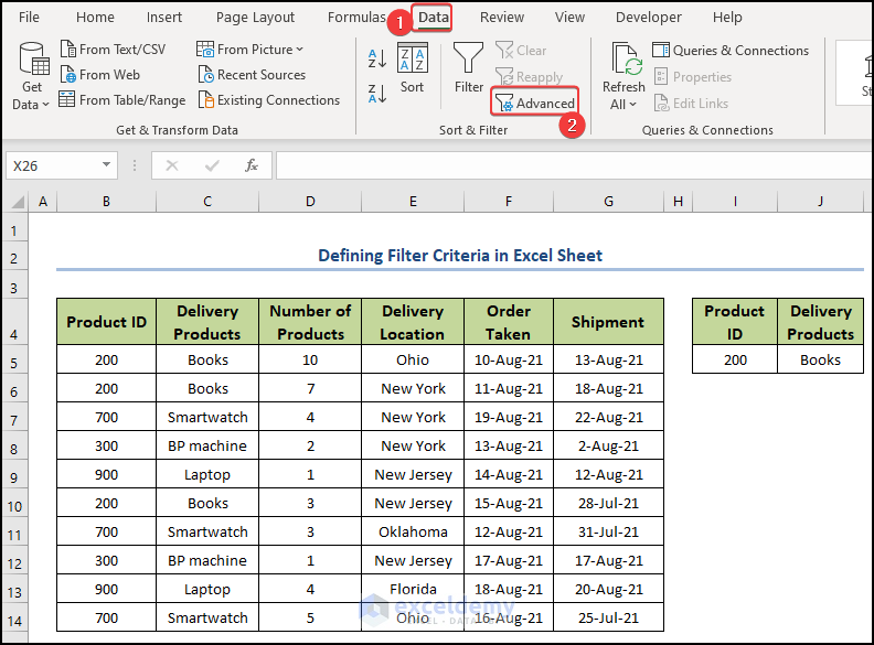
Method 5 – Defining Filter Criteria in Excel Sheet

Steps:

• Go to the Data tab.
• Click on the Advanced option from the Sort & Filter group.

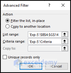
• A small dialog box called Advanced Filter will appear.
• Click on the List range field and select the range of cells B4:G14.
• Click on the Criteria range field and choose the range of cells I4:J5.
• Click OK.

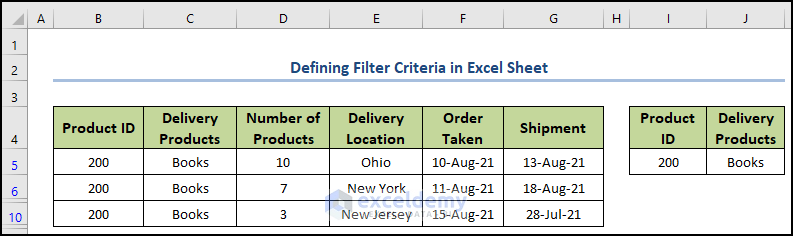
• You will get the following result.

Read More: How to Filter Data in Excel Using Formula

How to Clear an Existing Filter

Steps:

• Go to the sheet from where you want to remove the filter.
• In the Data tab, click on the Filter option from the Sort & Filter tab.

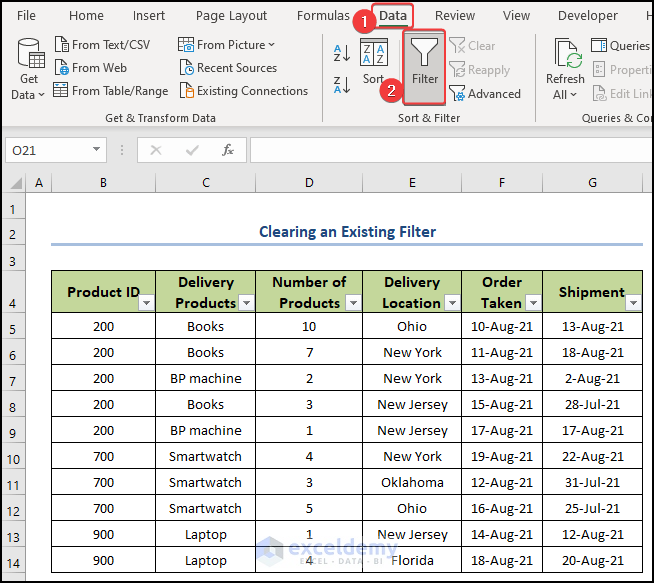
• The filter drop-down will disappear, and the filter will be cleared.

Read More: How to Remove Filter in Excel

Download the Practice Workbook

Download this workbook to practice.

<< Go Back to Data | Filter in Excel | Learn Excel