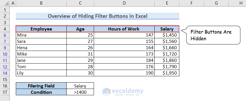
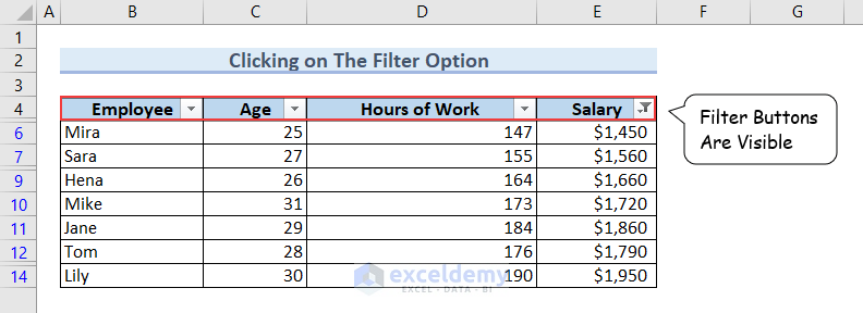
We often use Excel to maintain databases in our day-to-day life. In some cases, we need to filter our data based on specific conditions. This can be done easily in Excel. However, Filter buttons appear if you perform such filtering. Now if you don’t want the Filter button to be displayed, you can do that too. You may need that for a better presentation of your data. In this article, I’m going to demonstrate to you how to hide the Filter button in Excel. To get an overview of what it looks like, you may check the following image. In this image, we’ve performed filtering, but the Filter buttons are hidden.
How to Launch VBA Editor in Excel
As we’ll use the VBA environment throughout this work, we need to enable the VBA setup first if not done so.
Using Module Window:
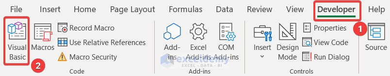
First of all, open the Developer tab. If you don’t have the developer tab, then you have to enable the developer tab. Then select the Visual Basic command.
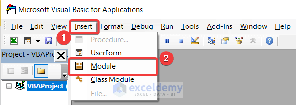
Hence, the Visual Basic window will open. Then, we’ll insert a Module from the Insert option where we’ll write the VBA Code.
How to Hide Filter Buttons in Excel: 6 Practical Examples
We need to perform filtering on our dataset based on certain conditions. For example, we have a dataset of Salaries. Our dataset looks like this.
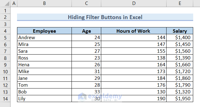
Our dataset contains information about Employee, Age, Hours of Work, and Salary. Now, we can filter the dataset based on a specific Salary condition. We’ve filtered the dataset based on Salary benign greater than $1400. Now we need to hide the filter buttons. To know how to hide filter buttons, now follow the descriptions.
1. Clicking Filter Option from Ribbon to Hide Filter Buttons
First of all, have a look at how our dataset looks when we’ve performed the filtering.
Now we need to hide the filter buttons.
- Click on cell E4 >> go to Data >> click on Filter as I’ve shown in the image.
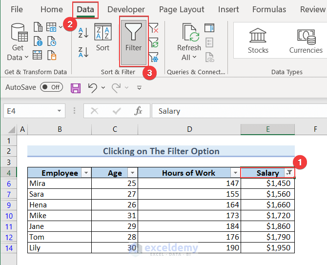
As a result, the Filter Buttons will be hidden.
2. Using Advanced Filtering to Filter Without Showing Buttons
We can use Advanced Filtering to filter the dataset based on our condition. This will filter the dataset according to the given condition and won’t show any Filter Button on the dataset at all.
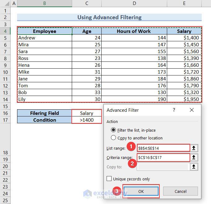
- Select cell B4 and go to Data >> Advanced Filter.
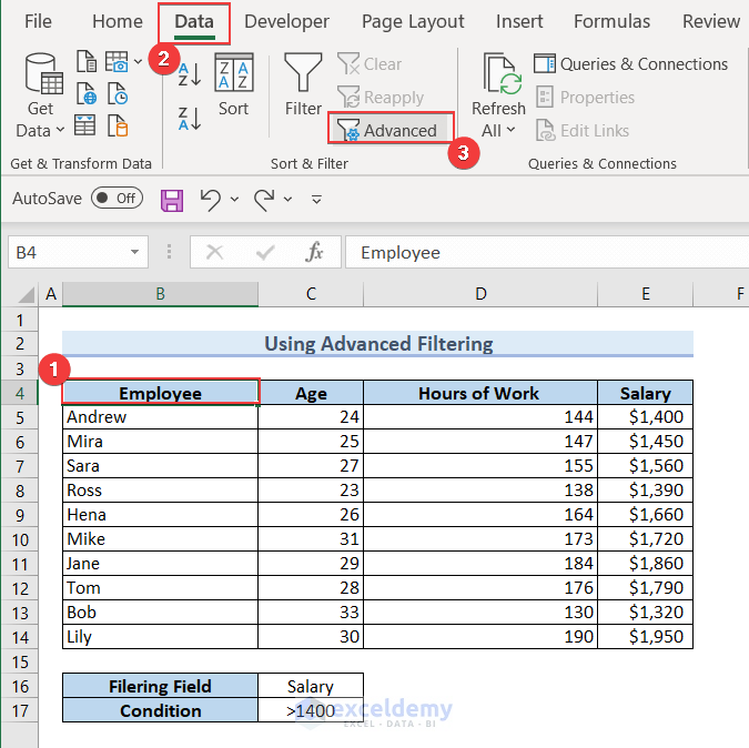
- Type $B$4:$E$14 in the List Range: to select the entire dataset to be filtered and $C$16:$C$17 in the Criteria Range: to get the dataset filtered based on a Salary greater than $1400. Finally, click on OK.
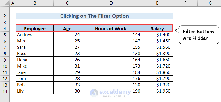
As a result, the data will be filtered based on the given criteria.
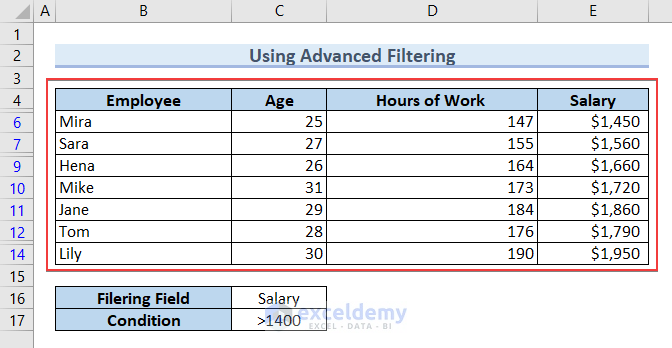
We can see from the image that no Filter Button is visible if we follow this method for filtering.
3. Using Excel VBA to Hide Filter Buttons
We can use the VBA to hide Filter Buttons in the filtered data. For example, our dataset looks like this.

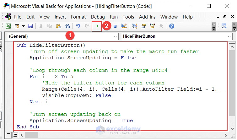
- Now, write the following VBA code to hide the Filter Buttons and click on the Run button.
Code:
Sub HideFilterButton()
'Turn off screen updating to make the macro run faster
Application.ScreenUpdating = False
'Loop through each column in the range B4:E4
For i = 2 To 5
'Hide the filter button for each column
Range(Cells(4, i), Cells(4, i)).AutoFilter Field:=i - 1, _
VisibleDropDown:=False
Next i
'Turn screen updating back on
Application.ScreenUpdating = True
End Sub
Code Breakdown:
Sub HideFilterButton()I’ve declared a subroutine named HideFilterButton that I’ll use to hide the Filter Buttons.
Application.ScreenUpdating = FalseThis statement turns off the ScreenUpdating feature. This improves the macro’s performance by preventing the screen from updating every time a change is made.
For i = 2 To 5
                        Range(Cells(4, i), Cells(4, i)).AutoFilter Field:=i - 1, _
                        VisibleDropDown:=False
            Next i
This set of statements runs a for loop that will run 4 times from column 2 to column 5. The variable i holds the current column number.
Then, the Cells function selects the current cell and hides the Filter Button of that cell by setting the VisibleDropDown to False.
Application.ScreenUpdating = TrueThis statement turns on ScreenUpdating so that we can see the change now.
End SubThis statement ends the subroutine.
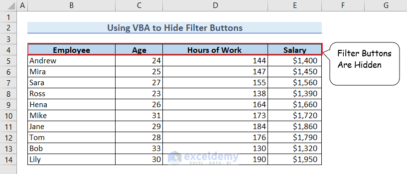
As a result, the Filter Buttons will be hidden from the worksheet.
4. Hiding Filter Buttons from Pivot Table
By default, Filter Buttons are displayed in the Pivot Table.
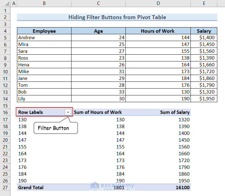
You can see the Filter Button in the following image. However, we can hide them if needed.
Now, we need to hide the Filter Button from the Pivot Table.
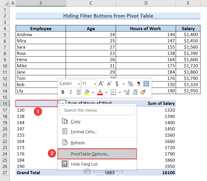
- Right-click on cell B16 and select the PivotTable Options.
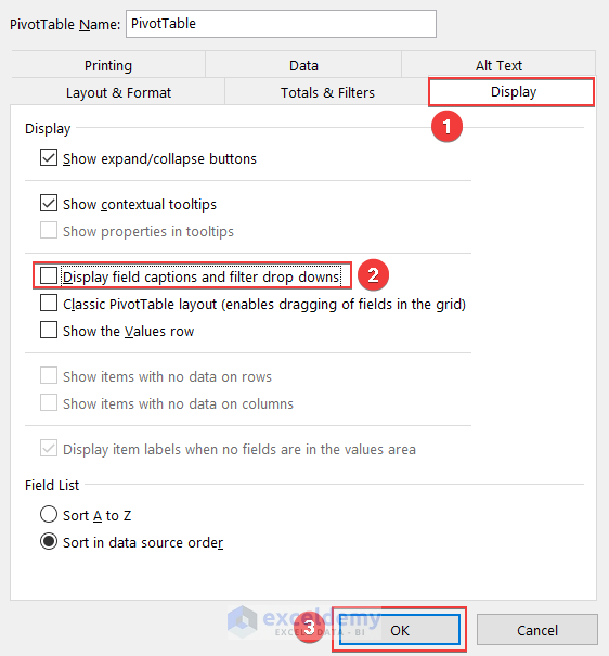
- PivotTable Options will now pop up. Navigate to Display and uncheck the Display field captions and filter drop downs. And click on OK.
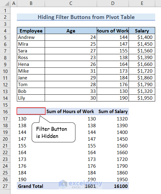
As a result, the Filter Button will be hidden in the Pivot Table.
5. Hiding Filter Buttons from Pivot Chart in Excel
Just like Pivot Table, Pivot Chart displays the Filter Button by default.
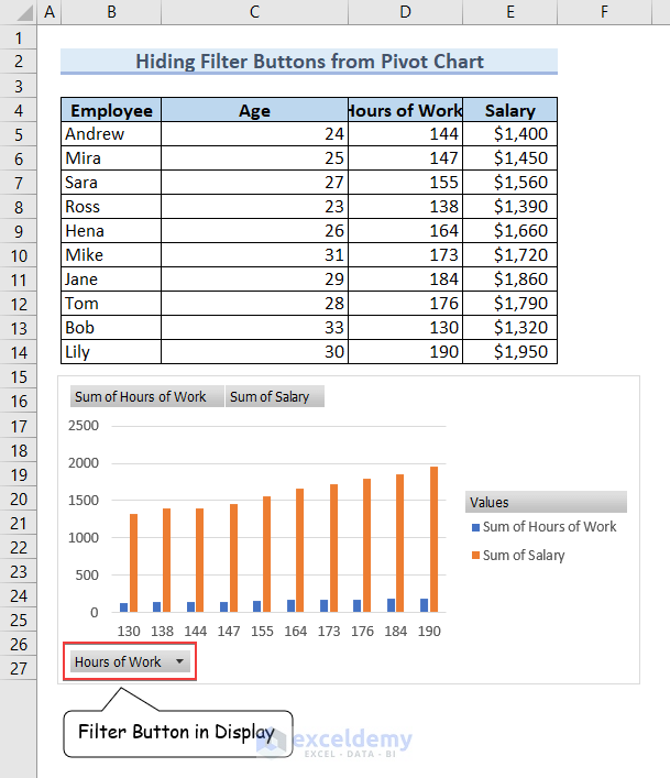
From the image, we can see the Filter Button is displayed in the Pivot Chart. Now, we need to hide the Filter Button from the Pivot Chart.
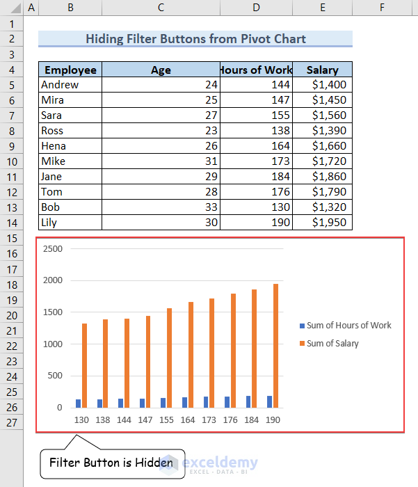
- Select the Pivot Chart >> Go to PivotChart Analyze >> Show/Hide >> Field Buttons >> Hide All.

Hence, the Filter Button will be hidden from the Pivot Chart. See the following image to check it.
Read More: How to Remove Filter in Excel
6. Hiding Filter Buttons from Table
If we convert a dataset into a Table, by default Filter Buttons appear on the Headers.

We can see Filter Buttons in the Table. We can hide the Filter Buttons from that Table too.
- Select Table1 from the Name Box to select the Table. Navigate to Table Design >> Table Style Options >> Filter Button and uncheck the Filter Button.
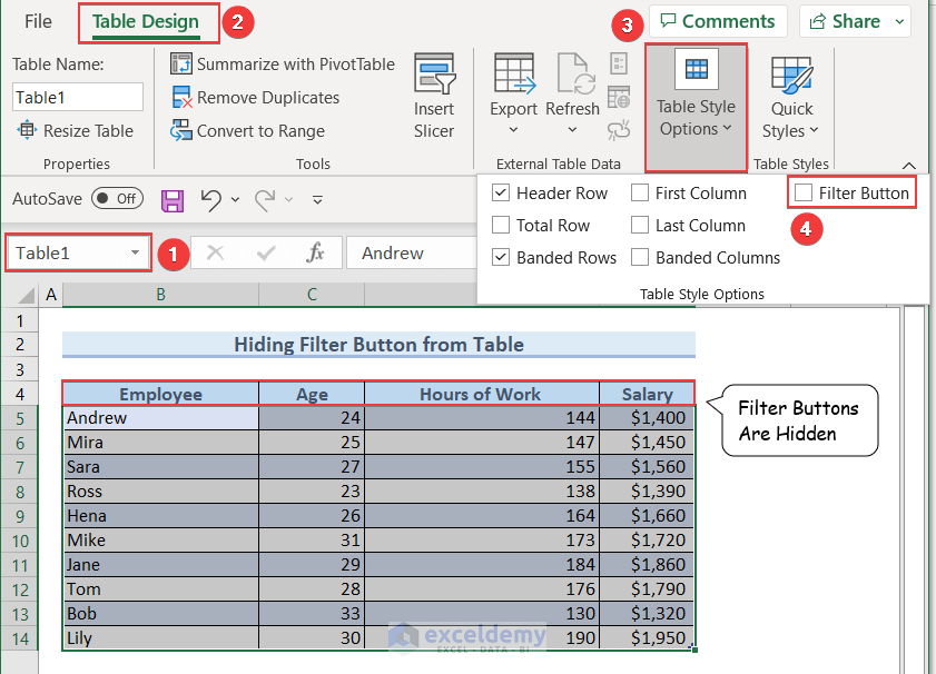
From the image, we can see that the FIlter Button is hidden now.
How to Unhide Pivot Table Filters in Excel
Pivot Table filters can be hidden sometimes. The following image shows such an example.
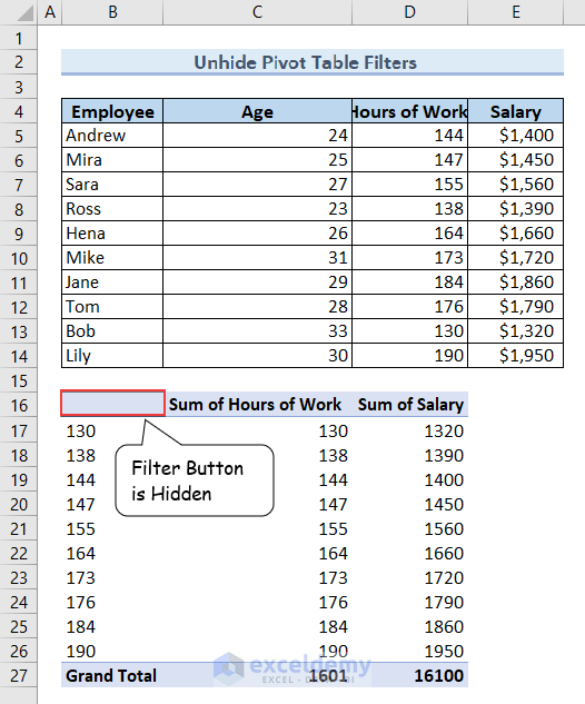
Now, we need to unhide the Filter Button in the Pivot Table.
- Right-click on cell B16 and select PivotTable.
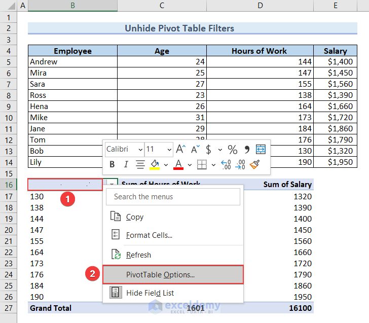
- PivotTable Options will now pop up. Navigate to Display and check the Display field captions and filter drop downs. And click on OK.
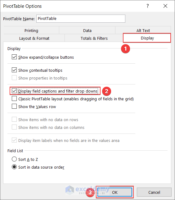
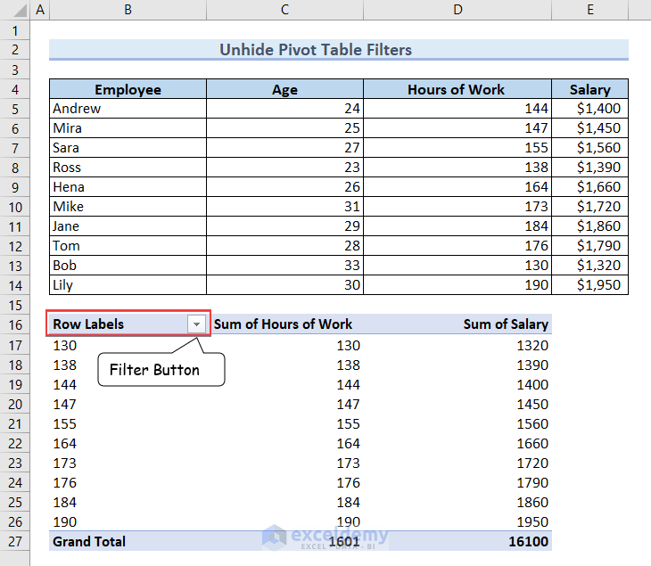
As a result, we can see that the Filter Button is visible in the Pivot Table.
How to Remove Filter Buttons from Some Columns in Excel
Sometimes you need to remove the Filter Buttons from some columns instead of removing them from all the columns. For example, our dataset looks like the following image.

We want to remove the Filter Buttons from the Employee and Hours of Work columns. We can do this using VBA.
- Write the following VBA code to hide the Filter Buttons and click on the Run button.

Code:
Sub HideFilterButtonFromSomeColumns()
'Turn off screen updating to make the macro run faster
Application.ScreenUpdating = False
'Loop through each column in the range B4:E4
For Each col In Range("B4:E4").Cells
'Hide the filter button for each column
col.AutoFilter Field:=1, VisibleDropDown:=False
col.AutoFilter Field:=3, VisibleDropDown:=False
Next col
'Turn screen updating back on
Application.ScreenUpdating = True
End Sub
Code Breakdown:
Sub HideFilterButtonFromSomeColumns()This statement declares a subroutine named HideFilterButtonFromSomeColumns.
Application.ScreenUpdating = FalseThis statement turns off the ScreenUpdating option.
For Each col In Range("B4:E4").Cells
col.AutoFilter Field:=1, VisibleDropDown:=False
col.AutoFilter Field:=3, VisibleDropDown:=False
Next col
This set of statements hides the VisibleDropDown that is the Filter Buttons from cell B4 and D4. Note that, the argument of FIeld is 1 to indicate column B and 3 to indicate column D.
Application.ScreenUpdating = TrueThis statement turns on ScreenUpdating so that we can visualize that the Filter Buttons are hidden from the mentioned columns.
End Sub This statement ends the subprocedure.
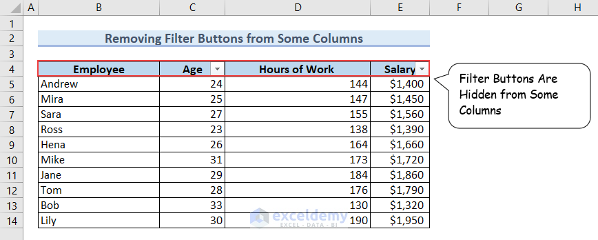
As a result, the Filter Buttons will be hidden from the columns Employee and Hours of Work. We can see it in the following image.
Takeaways from This Article
If you’ve followed this article thoroughly, you’ll be now able to:
- Hide the Filter Buttons from Table, Pivot Chart, Pivot Table, etc whenever necessary.
- Hide Filter Buttons from some specified columns.
- Unhide the Filter Buttons.
Things to Remember
While working on VBA to hide the Filter Buttons, keep in mind to refer to the cells properly.
- You should adjust my code properly to hide Filter Buttons from your dataset.
- Use correct references while using the Advanced Filter option.
Download Practice Workbook
You can download our practice workbook from here for free!
Conclusion
I’ve demonstrated how to hide filter buttons in Excel throughout this article. I’ve shown the real-life use cases of hiding the Filter button from the Table, Pivot Chart, Pivot Table, and dataset. You may apply this in your own situations according to your needs. If you wish to keep the filtering intact, I would recommend using the Advanced Filter option that I’ve demonstrated here. I hope you’ll now be able to hide the Filter button easily.
If you face any problems implementing these methods or if you face any other Excel issues, let us know in the comment section. I’ll try to solve your problem. Thanks for following along with me. Have a good day!
<< Go Back to Filter in Excel | Learn Excel
Get FREE Advanced Excel Exercises with Solutions!
