The following GIF shows the filtered rows based on the device name from the drop-down selection, which we’ll create.
Method 1 – Apply Keyboard Shortcuts to Filter Data Based on Cell Value
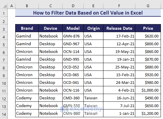
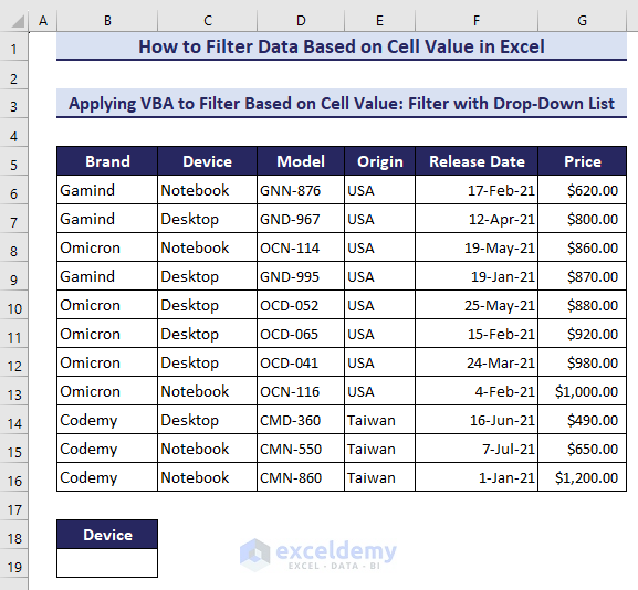
Our dataset contains PC brands, device types, model names, origins, release dates, and corresponding prices.
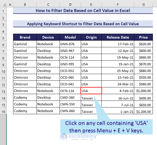
- Select a cell for which value you want to filter your dataset. We’ll filter for the origin country being USA.
- Press and hold the Menu key on your keyboard and press E + V.
- The Filter command will be activated and it will show the filtered rows based on your selection.
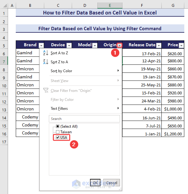
Method 2 – Filter Data Based on Cell Value by Using the Filter Command
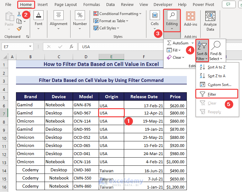
- Select any cell of your dataset.
- Go to Home then to Editing.
- Choose Sort & Filter and pick Filter.
- The Sort & Filter icon will be visible in every header of your dataset.
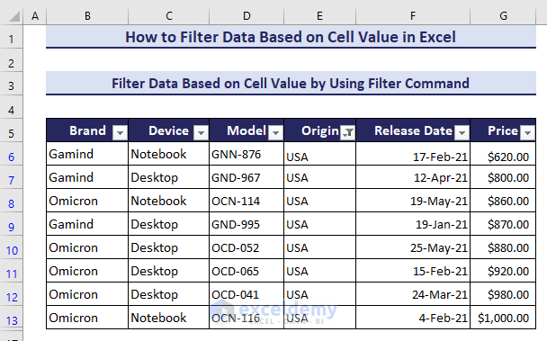
- Click on the Sort & Filter icon of the Origin header and mark USA from the list.
- Here’s the filtered result.
Method 3 – Apply the FILTER Function to Filter Data Based on Cell Value
Example 1 – Filter for a Range
We’ll filter the data based on a price range of $700 to $1,000.
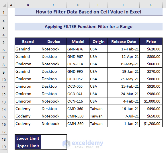
- Insert the following formula in cell B22 and hit the Enter button:
=FILTER(B6:G16, (G6:G16 >C18 )*(G6:G16<C19))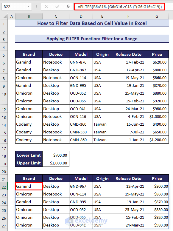
- If you change the values, it will instantly update the filter result as shown below.
Example 2 – Filter for Specific Text
Let’s filter the data for model names that contain the term ocd.
- Apply the following formula in cell B21 and press the Enter button:
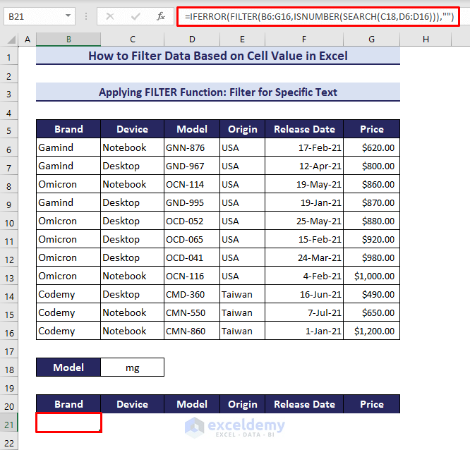
=IFERROR(FILTER(B6:G16,ISNUMBER(SEARCH(C18,D6:D16))),"")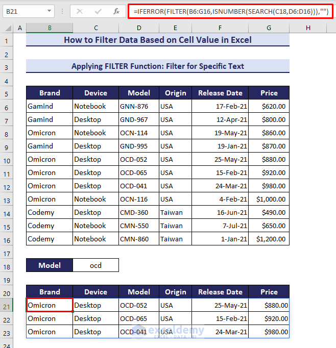
- Whenever you type a text partially, it will return the matched result.
- The IFERROR function avoids the #CALC! error and will return a blank.
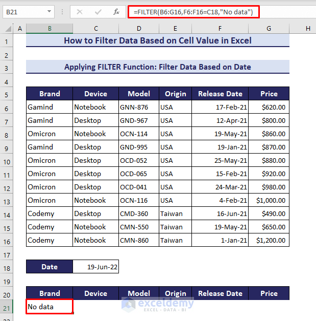
Example 3 – Filter Data Based on Date
- Use the following formula in cell B21 to filter the data for the date 19-May-21:
=FILTER(B6:G16,F6:F16=C18,"No data")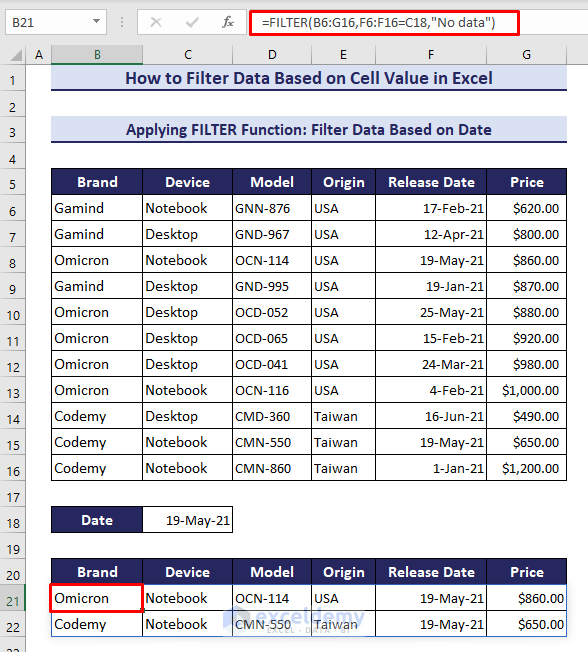
- If the date doesn’t match with any date of our dataset, the function will return No Data.
Example 4 – A Dynamic Filter with a Drop-Down List
- Insert the following formula in cell B21 to filter the data by Desktop, which is in cell C18.
=FILTER(B6:G16,ISNUMBER(SEARCH(C18,C6:C16)))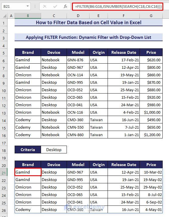
- We created a drop-down list by using the Data Validation tool to get dynamic results.
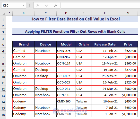
Example 5 – Filter Out Rows with Blank Cells
We modified the dataset by keeping some blank cells in some rows.
- Insert the following formula in cell B19 and press Enter to filter out the rows with blank cells:
=FILTER(B6:G16,(C6:C16<>"")*(D6:D16<>""),"No Result")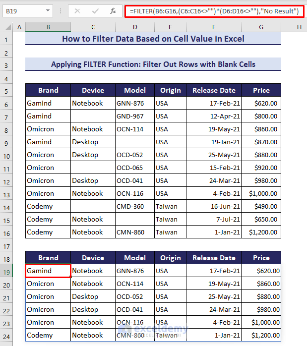
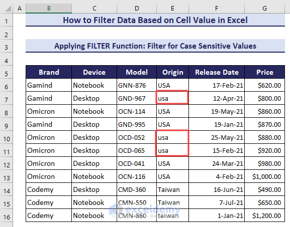
Example 6 – Filter for Case-Sensitive Values
In the Origin column, there are two types of cases for the same origin, “USA” and “usa”.
- Apply the following formula in cell B21 to filter the data for lowercase “usa”:
=FILTER(B6:G16,EXACT(E6:E16,C18))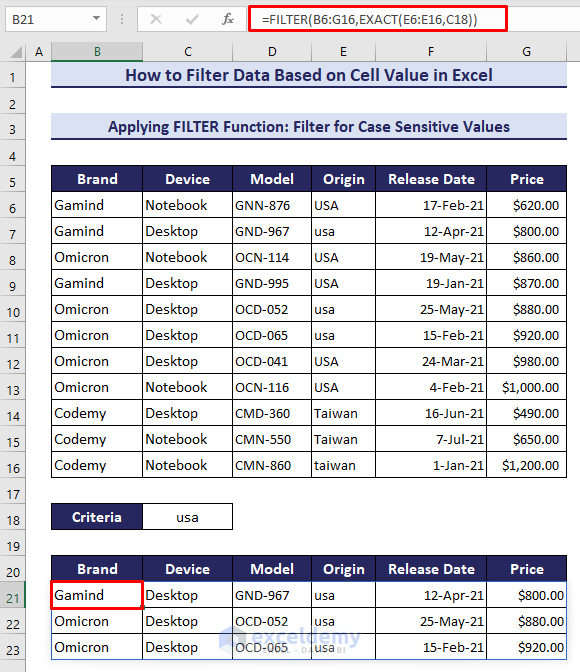
- Here’s the result.
Method 4 – VBA Code to Filter Data Based on Cell Value
Case 1 – Filter for Top N Values
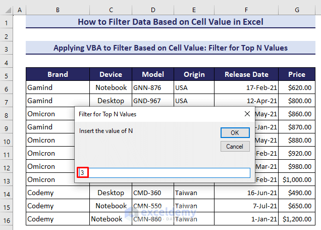
We’ll filter the data for top N values from the Price column.
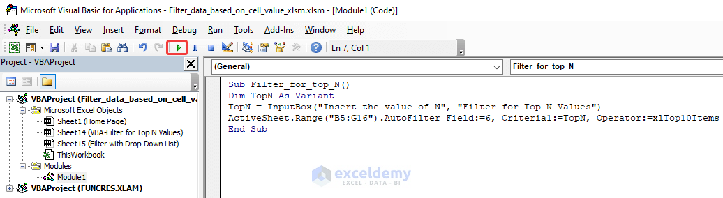
- Insert the following code in a new Module:
Sub Filter_for_top_N()
Dim TopN As Variant
TopN = InputBox("Insert the value of N", "Filter for Top N Values")
ActiveSheet.Range("B5:G16").AutoFilter Field:=6, Criteria1:=TopN, Operator:=xlTop10Items
End Sub- Run the code by clicking on the Run icon or by pressing F5.
- An input box will open up to insert the value of N. We inserted 3.
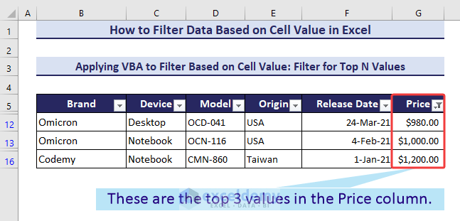
- The dataset will be filtered based on the top 3 values of the Price column.
Case 2 – Filter with a Drop-Down List
We’ll create the drop-down list in cell B19.
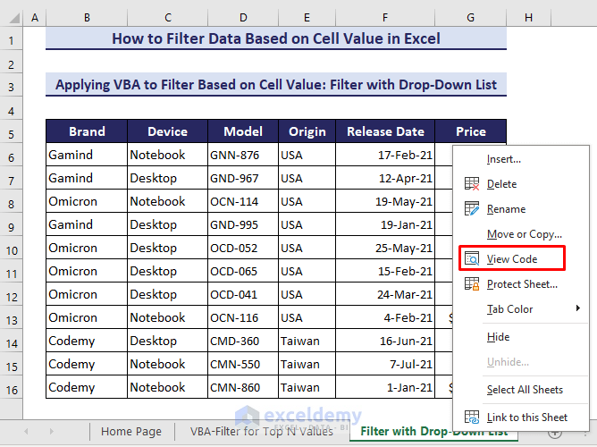
- Right-click on the sheet name.
- Select View Code from the context menu.
- Put in the following code:
Private Sub Worksheet_Change(ByVal Target As Range)
If Target.Address = Range("B19").Address Then
Range("B5:G16").CurrentRegion.AdvancedFilter Action:=xlFilterInPlace, CriteriaRange:=Range("B18:B19")
End If
End Sub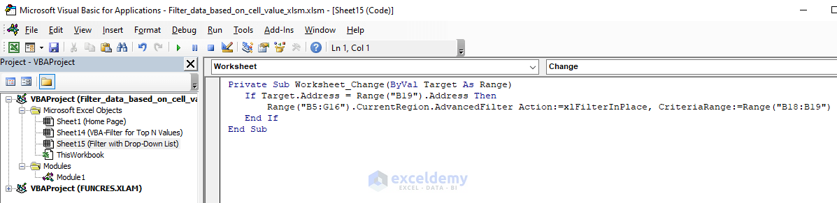
- If we change the value in cell B19, the VBA code will automatically filter the data range according to that value.
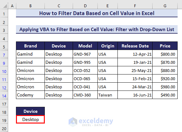
- We added a drop-down list in cell B19 for easy selection.
Download the Practice Workbook
<< Go Back to Data | Filter in Excel | Learn Excel
Get FREE Advanced Excel Exercises with Solutions!
