How to Filter Multiple Rows in Excel: 11 Suitable Methods

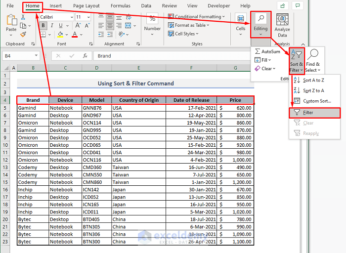
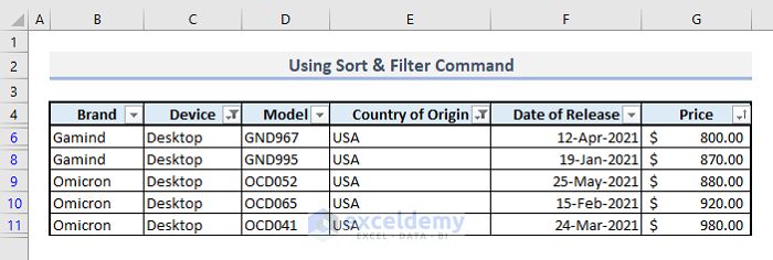
Method 1 – Using Sort and Filter Command to Filter Multiple Rows

Step 1:

➤ Select the headers of the table.

➤ Under the Home tab, select the Filter command from the Editing and Sort and Filter drop-down. You’ll see the filter buttons in your table headers now.

Step 2:

➤ From the Country of Origin options, select USA only.

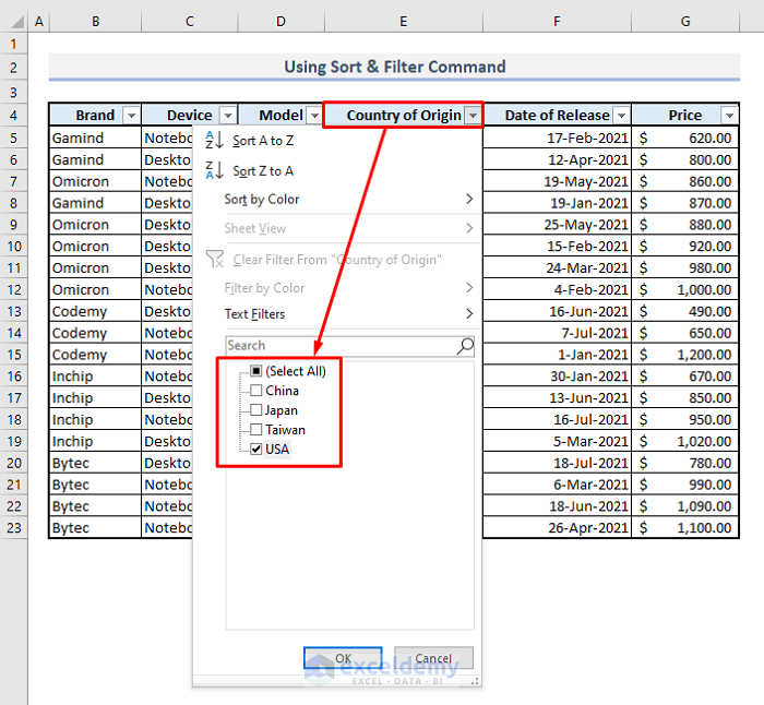
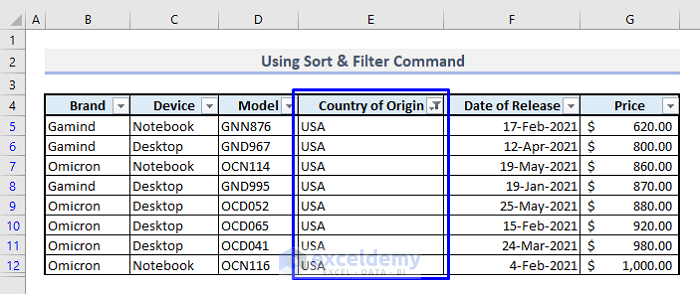
Press Enter and you’ll find all the devices originated in the USA.

Step 3:

➤ Select Desktop from the Device menu.

➤ Press OK.

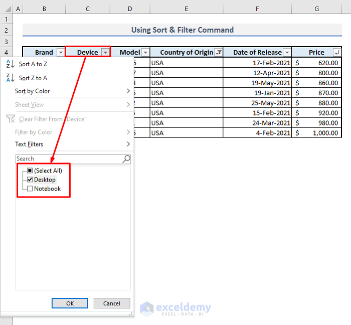
You’ll be displayed all the columns based on two selected criteria at once. You’ve just got all the available data for desktop devices made in the USA.

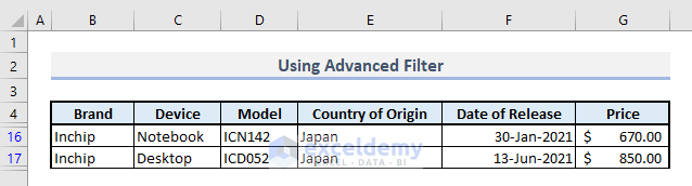
Method 2 – Applying Advanced Filter for Multiple Rows

Step 1:

➤ From the Data ribbon, select the Advanced command from the Sort and Filter group of commands. A dialogue box will appear.

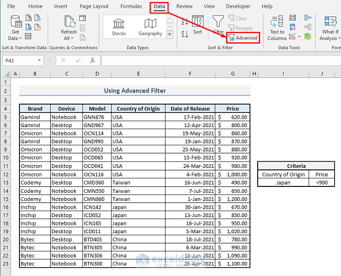
Step 2:

➤ Select the entire table or the array- B4:G23 for the List Range.

➤ Select Criteria table or the range of Cells- I12:J13 for Criteria Range.

➤ Press OK.

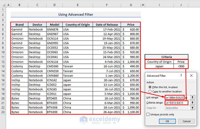
You’ll be shown the filtered table based on the selected criteria.

Method 3 – Using Autofilter to Customize Filter for Multiple Rows

Step 1:

➤ Assign the Filter buttons to all headers.

➤ From the Price menu, select the Custom Filter option from the Number Filter drop-down.

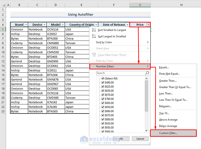
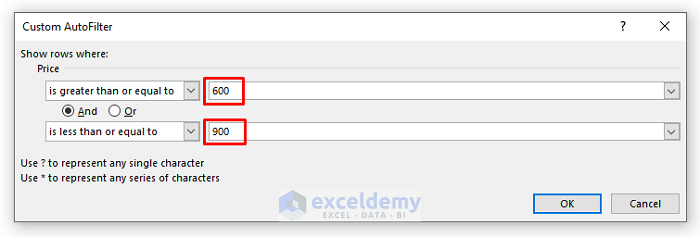
Step 2:

➤ In the AutoFilter dialogue box, select the 1st price criteria as ‘Is greater than or equal to’ and then type 600 as the value for this criteria.

➤ Select the 2nd price criteria as ‘Is less than or equal to’ and input the value as 900 for this criteria.

➤ Press OK.

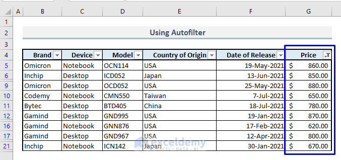
Get the following result with the Price column filtered.

Method 4 – Inserting FILTER Function to Filter Multiple Rows with Criteria

Before getting down to the uses of the FILTER function, we can have a look at how this function works.

• The Objective of the Function:

Filter a range or an array.

• Syntax:

=FILTER(array, include, [if_empty])

• Arguments:

array- Array or range of cells that has to be filtered.

include- Criteria for the function.

[if_empty]- It’s optional. If the function finds nothing from the data the message will be shown based on the texts inputted here.

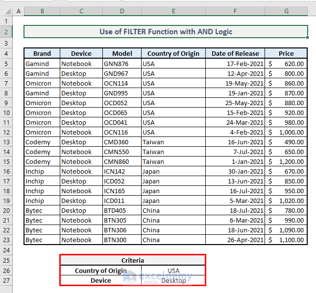
4.1 Filtering Multiple Rows with AND Criteria

Based on our dataset, we’ll filter the devices and origin countries only. We’re adding two different criteria from two different columns here.

Steps:

➤ Select the output Cell B30 and type:

➤ Press Enter and you’ll get the resultant array for desktops made in the USA only.

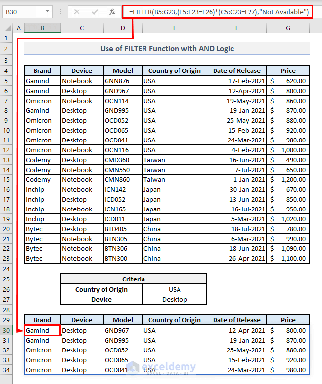
In this function, you have to add two or more criteria by using Asterisk(*) among them in the 2nd argument.

4.2 Filtering Multiple Rows with OR Criteria

Now we’ll add two different criteria for the same column. We’ll find out all the available data from the table for two origin countries: Japan and Taiwan.

Steps:

➤ Select Cell B30 and type:

➤ Press Enter and you’ll get the filtered array right away.

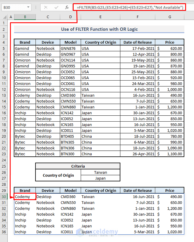
Add multiple OR logic, you have to use the Plus(+) symbol between two criteria in the 2nd argument.

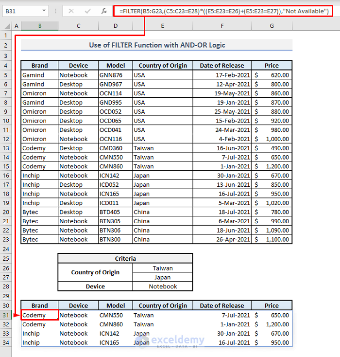
4.3 Filtering Multiple Rows with AND-OR Criteria

Steps:

➤ In Cell B31, the related formula will be:

➤ Press Enter and you’ll get the return values.

Method 5 – Filtering Duplicates from Multiple Rows

Steps:

➤ Select Cell B26 and type:

➤ Press Enter.

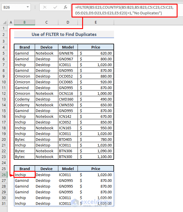
How Does This Formula Work?

➤ The COUNTIFS function searches for all duplicates and then counts those findings.

➤ FILTER function then searches for the counts that are more than 1 and accordingly shows the data from the original table.

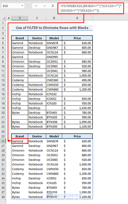
6. Filtering Out Rows Containing Blank Cells

Steps:

➤ In Cell B26, the related formula will be:

➤ After pressing Enter, you’ll get the filtered result at once.

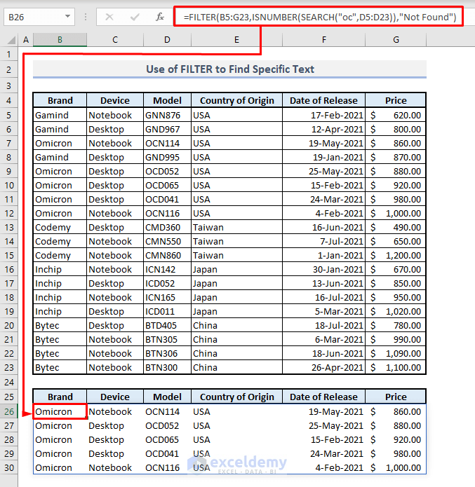
Method 7 – Filtering Multiple Rows to Find Specific Text

Steps:

➤ Select the output Cell B26 and type:

➤ Press Enter and you’ll get all the data for the selected brand names with specific texts “oc”.

How Does This Formula Work?

➤ SEARCH function searches for the text “oc” in Column B and returns with ‘1’ for each finding.

➤ ISNUMBER identifies the numbers or all 1’s found from the SEARCH results and returns with the logical values- TRUE or FALSE.

➤ The FILTER function shows all the available data from the table based on the row numbers of the logical values- TRUE found from the previous step.

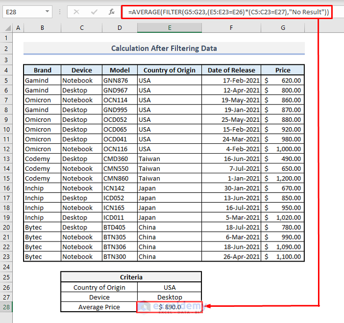
Method 8 – Filtering Multiple Rows for Calculation

Steps:

➤ Select the output Cell E28 and type:

➤ Press Enter and you’ll be shown the evaluated result based on the filtered data at once.

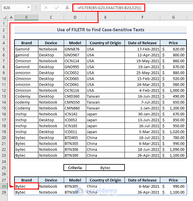
Method 9 – FILTER function for Case-sensitive Text Strings from Multiple Rows

Steps:

➤ The related formula in Cell B28 will be:

➤ Press Enter and the resultant array with Bytec only will be displayed.

Method 10 – Filtering Multiple Rows for Specific Columns

Steps:

➤ In Cell I14, the related formula will be:

➤ Press Enter and you’ll be shown the specific columns only with selected criteria.

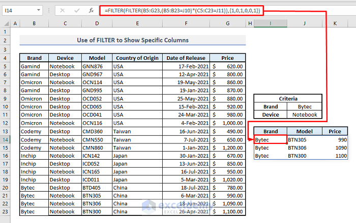
The outer FILTER function shows the specific columns based on the presence of 1 in the array of {1,0,1,0,0,1} in the 2nd or ‘include’ argument.

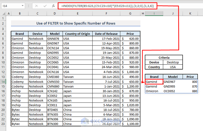
Method 11 – Showing Specific Number of Rows from Multiple Rows with FILTER Function

Steps:

➤ Select the output Cell I14 and type:

➤ Press Enter and you’ll find your customized table of data right away.

Download Practice Workbook

You can download the Excel workbook that we’ve used to prepare this article.