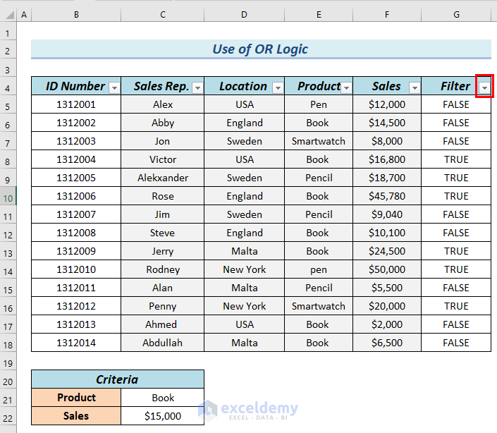
In the following dataset, you can see the ID Number, Sales Rep., Location, Product, and Sales columns. We’ll filter the results by multiple columns.
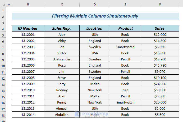
Method 1 – Using the Filter Option to Filter Multiple Columns Simultaneously in Excel
We will filter columns C and D to find the names that start with the letter A and whose location is USA.
Steps:
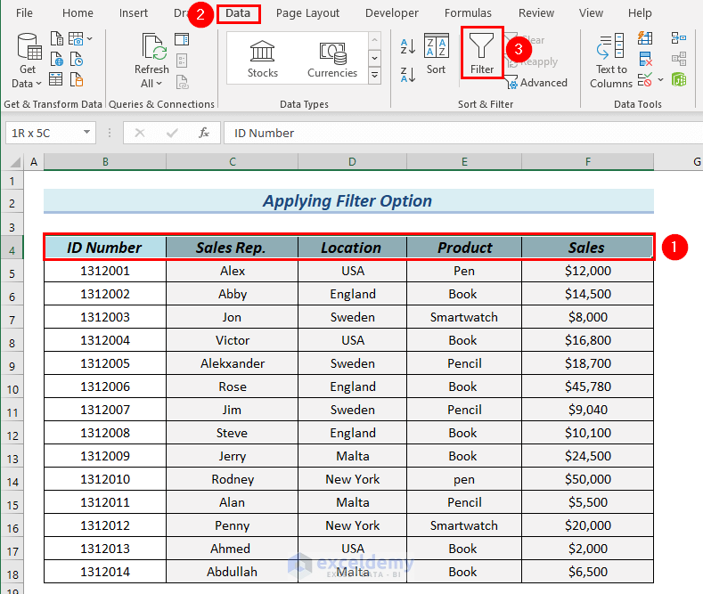
- Select the header of the data table by selecting cells B4:F4 to apply the filter option.
- Go to the Data tab.
- From the Sort & Filter group, select the Filter option.
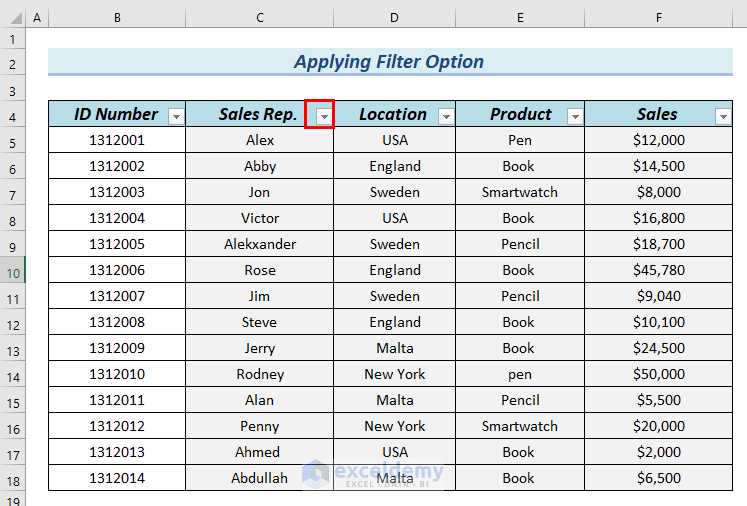
- Click on the Filter icon of column C.
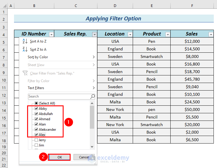
- Select the names that start with A and unmark the other names.
- Click OK.
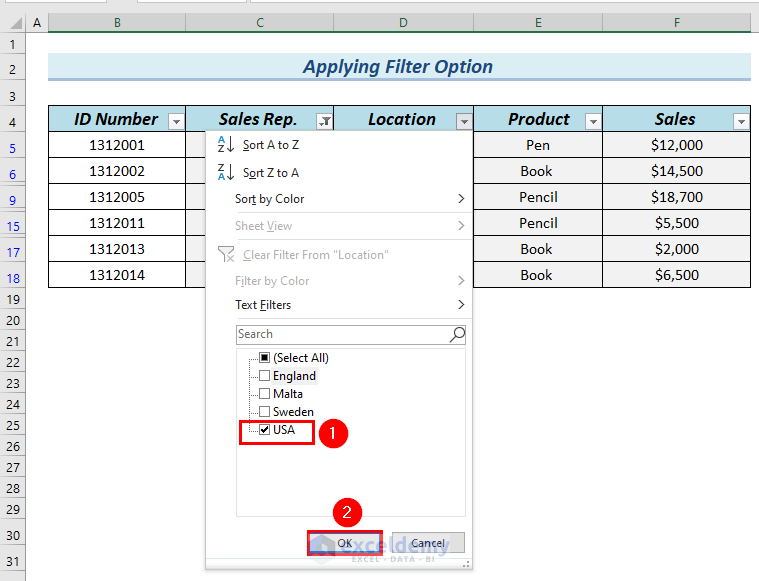
- Click on the Filter icon of column D.
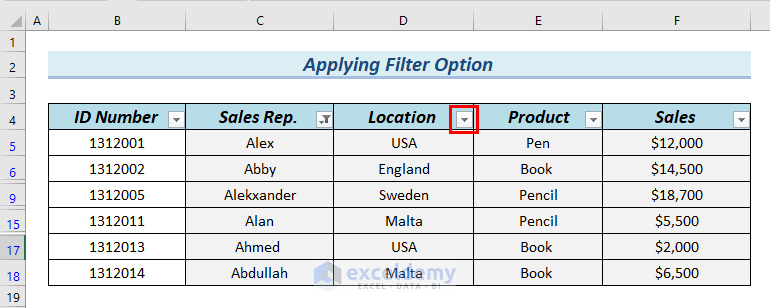
- Mark USA and unmark the other locations.
- Click OK.
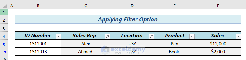
- The dataset is now showing the data of names that start with A and that are present in the USA.
Read More: How to Filter Multiple Columns Independently in Excel
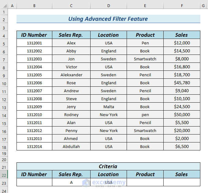
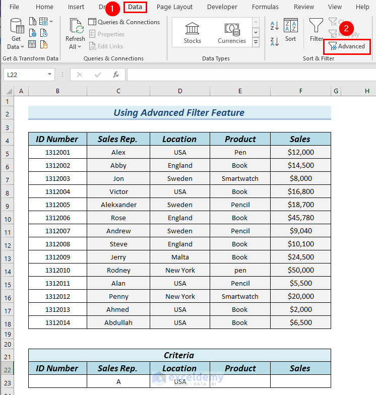
Method 2 – Using the Advanced Filter Feature to Filter Multiple Columns Simultaneously in Excel
We want to filter the names that start with A with the location USA. You can see these criteria in the Criteria box.
Steps:
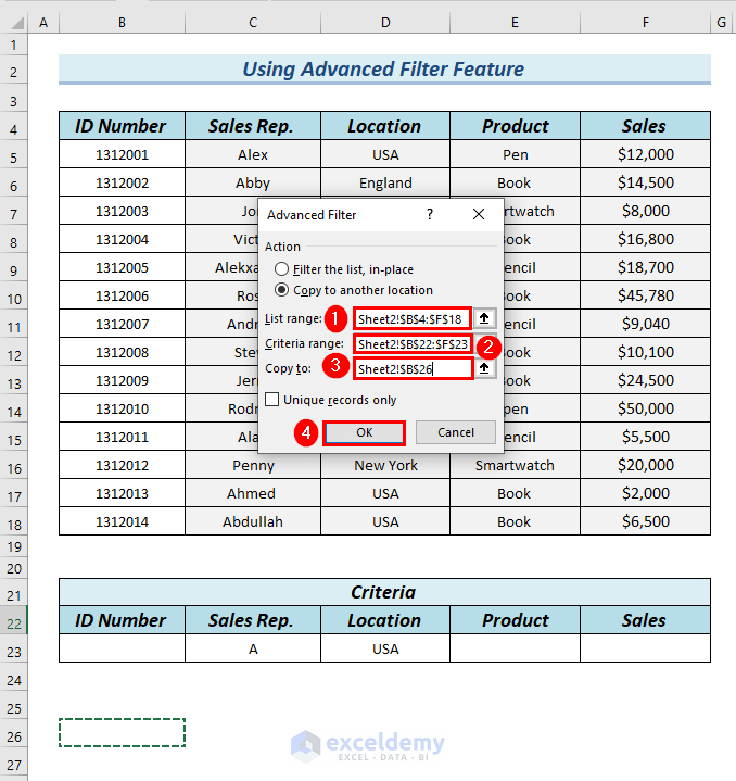
- Go to the Data tab and, from the Sort & Filter group, select Advanced Filter.
- In the Advanced Filter dialog box, select cells B4:F18 as List Range.
- Select cells B22:F23 as Criteria range.
- Select Copy to another location and select cell B26 in the Copy to box.
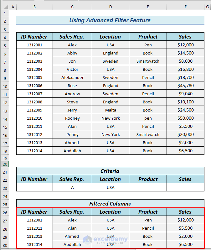
- Click OK.
- Here are the results.
Read More: How to Search Multiple Items in Excel Filter
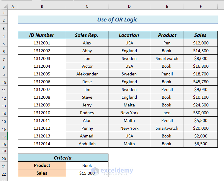
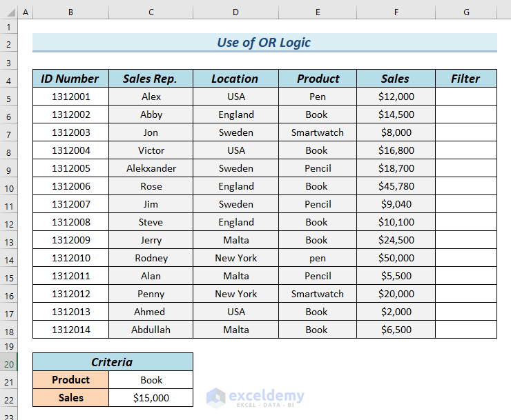
Method 3 – Using OR Logic to Filter Multiple Columns Simultaneously in Excel
We need to filter column E by Book and column F by values greater than 15,000. You can see the criteria in the Criteria table.
Steps:
- Add a column G named Filter to the dataset.
- Enter the following formula in cell G5.
=OR(E5=$C$21,F5>$C$22)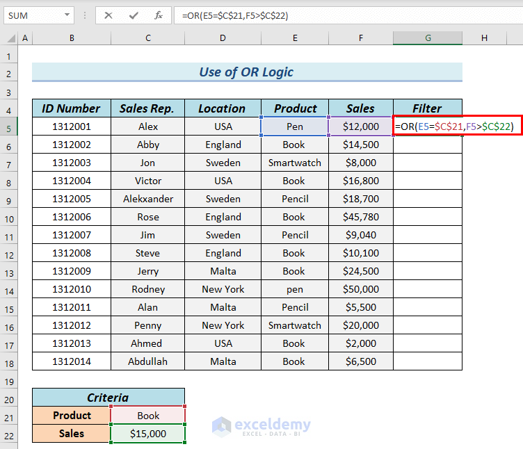
Formula Breakdown
- OR(E5=$C$21,F5>$C$22) → the OR Function determines whether any logical tests are true or not.
- E5=$C$21 → is logical test 1
- F5>$C$22 → is logical test 2
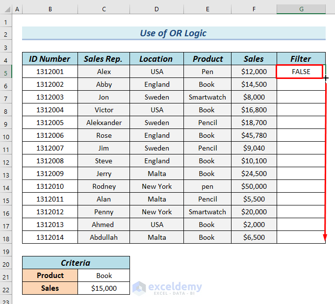
- Output: FALSE
- Explanation: Since none of the logical tests are true, the OR function returns FALSE.
- Press Enter.
- Drag down the formula with the Fill Handle tool.
- Select the header of the data table, i.e. cells B4:F4.
- Go to the Data tab.
- From the Sort & Filter group, select the Filter option.
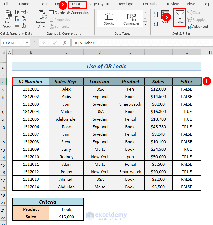
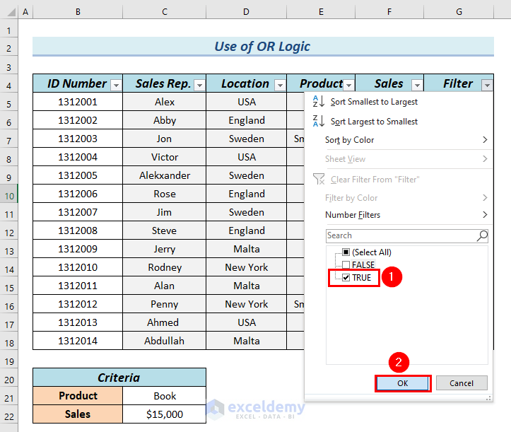
- Click on the Filter icon of column G to filter the values TRUE from column G.
- Mark TRUE and unmark FALSE.
- Click OK.
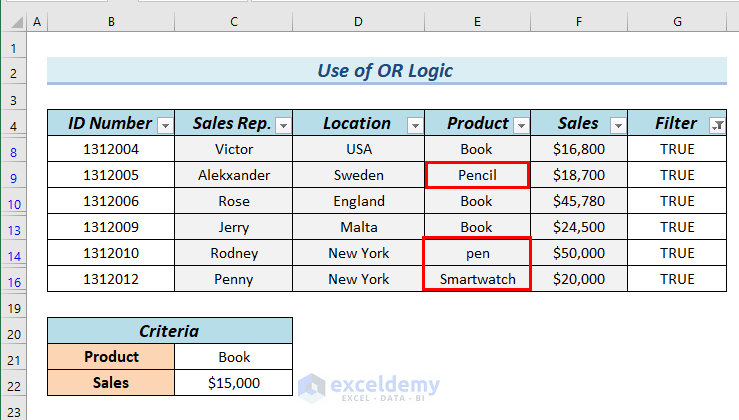
- Here are the results.
Read More: How to Filter Data in Excel Using Formula
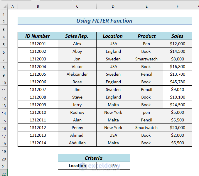
Method 4 – Using the FILTER Function to Filter Multiple Columns Simultaneously in Excel
We will filter the dataset based on the location USA as shown in the Criteria table.
Steps:
- Enter the following formula in cell B24.
=FILTER(B5:F18,D5:D18=D5,"")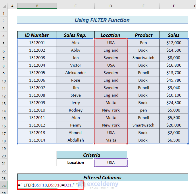
Formula Breakdown
- FILTER(B5:F18,D5:D18=D5,” “) → the FILTER function filters a range of cells based on criteria.
- B5:F18 → is the array.
- D5:D18=D5 → is the criteria
- ” ” → returns a blank cell when the criteria are not met.
- Press Enter.
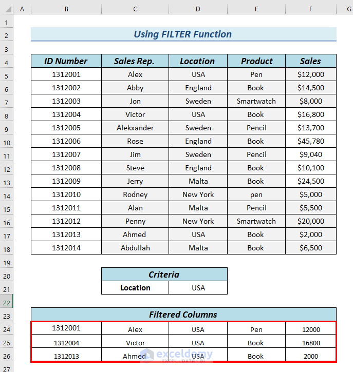
Read More: How to Filter Column Based on Another Column in Excel
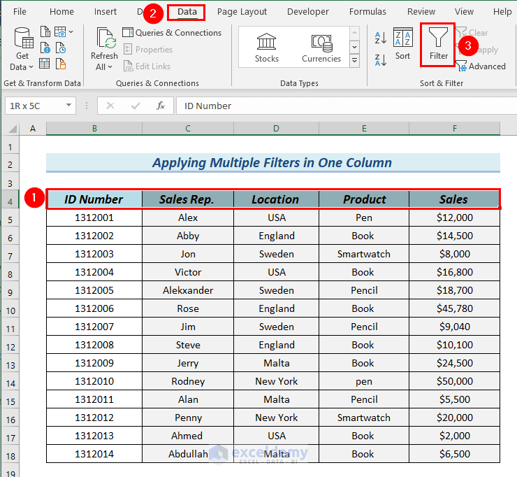
How to Apply Multiple Filters in One Column in Excel
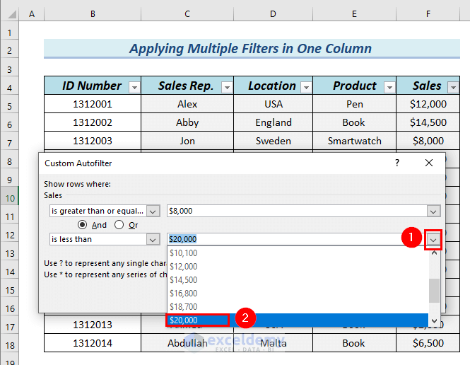
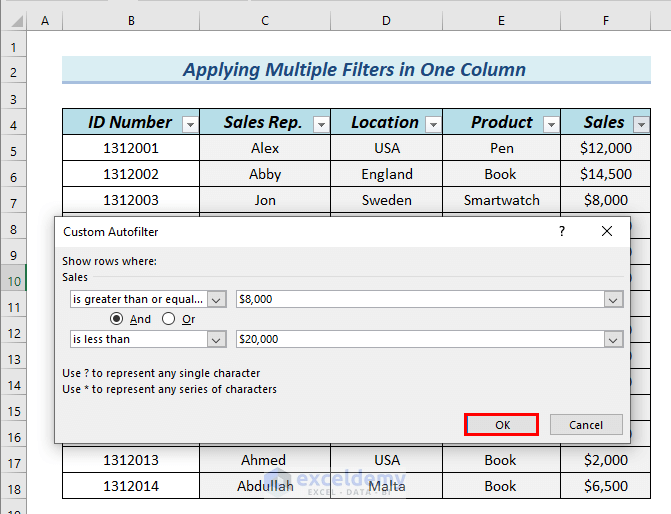
We want to find the Sales values that are greater than or equal to $8,000 and lower than $20,000.
Steps:
- Select the column headings B4:F4.
- Go to the Data tab.
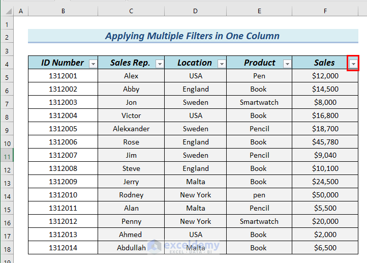
- From the Sort & Filter group, select the Filter option.
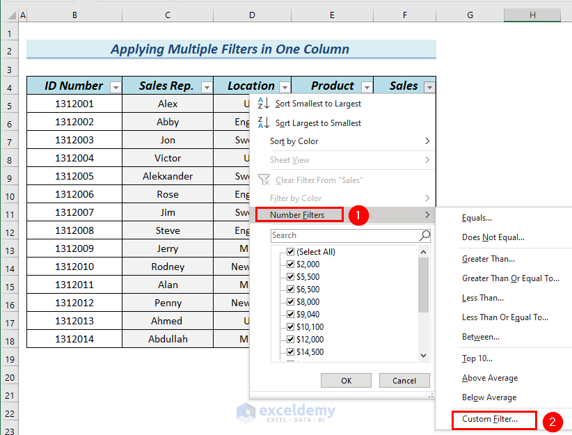
- Click on the Filter icon of column F.
- Select Number Filters then choose Custom Filters.
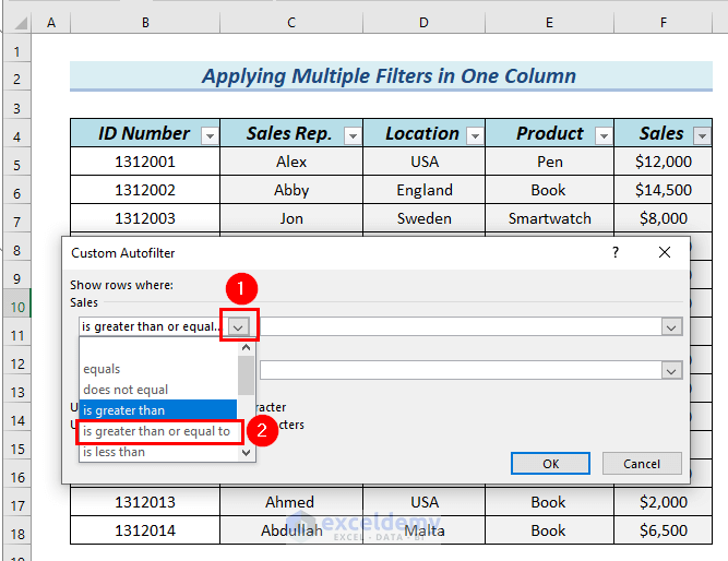
- A Custom Autofilter dialog box will appear.
- Click on the drop-down of the first box.
- Select the option is greater than or equal to.
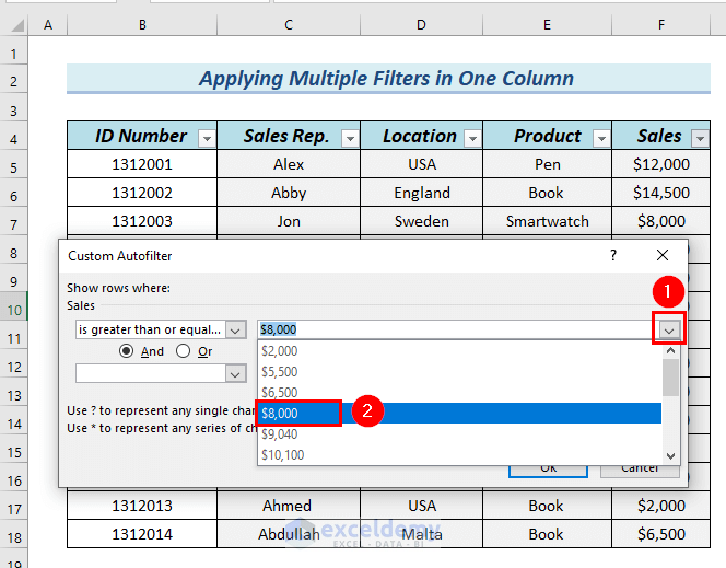
- Select $8,000.
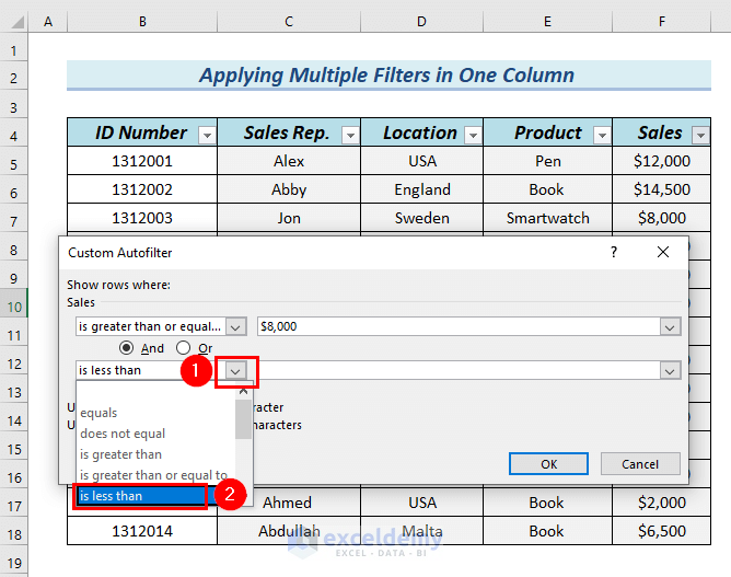
- Click on the drop-down arrow of the second box.
- Select the option is less than.
- Select $20,000.
- Click OK.
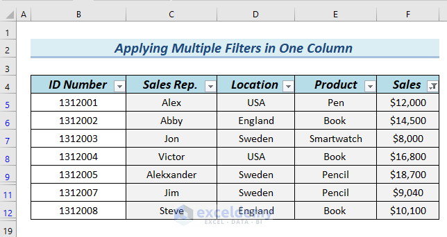
- Here’s the filtered Sales column.
Things to Remember
- While using the advanced filter tool, you can choose Filter in the list to filter the data in the same place where you select the range.
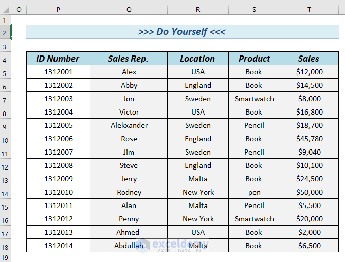
Practice Section
We have included a practice dataset you can use to test the methods.
Download the Practice Workbook
<< Go Back to Data | Filter in Excel | Learn Excel
Get FREE Advanced Excel Exercises with Solutions!

I can get advance filter to work with St = FL or with Memb Notes = *FL-Seasonal* (in proper criteria cells) but not with both together.
Hello JN,
To make the Advanced Filter work with both criteria (e.g., St = FL and Memb Notes = *FL-Seasonal*), you need to arrange the criteria in a specific way:
1. Place the conditions for AND logic (both must be true) in the same row.
2. Place the conditions for OR logic (either can be true) in separate rows.
For your case:
If you want both conditions to apply simultaneously (AND logic), ensure they are in the same row under their respective headers in the criteria range.
If you’re facing issues, double-check the formatting of the criteria, such as using =”=FL” for exact matches or wildcard symbols like * for partial matches.
Regards
ExcelDemy