Excel Doughnut Chart

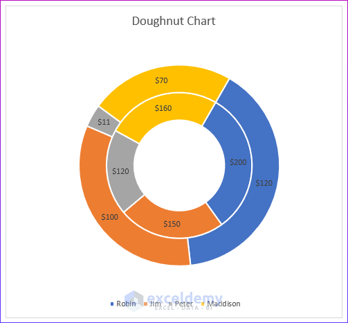
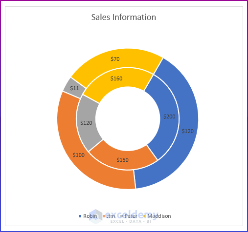
Here’s an example of a donut chart with multiple rings.

Download the Practice Workbook

Excel Doughnut Chart.xlsx

What Exactly Is a Doughnut Chart?

Doughnut charts show each cell’s data as a slice of doughnut. One or more doughnuts may be stacked on top of each other on the chart. Doughnut charts show the link between several types of data. Each doughnut presents a different piece of data.

What Are the Examples of Creating a Doughnut Chart in Excel?

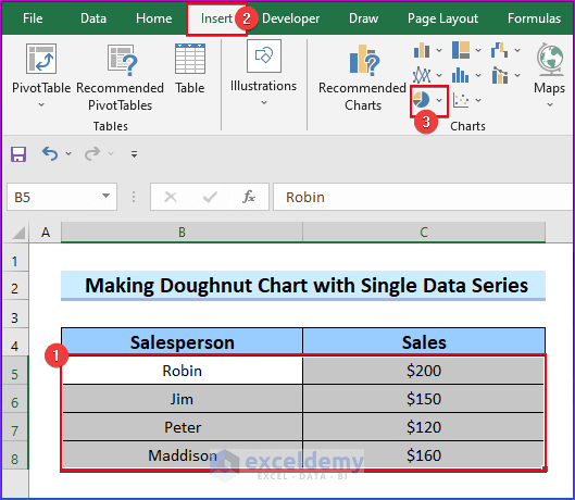
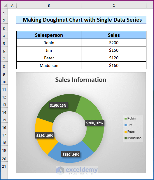
Example 1 – Making a Doughnut Chart with a Single Data Series

Select the dataset that you want to include in your doughnut chart.
Go to the Insert tab.
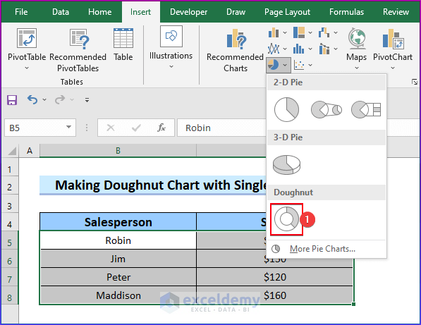
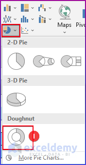
Select Insert Pie or Doughnut Chart from the Charts options.

From the drop-down menu, choose Doughnut chart.

You will see a doughnut chart in your worksheet.

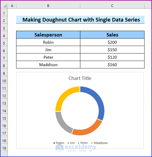
Double-click on the Chart Title. You can type the relevant title of the chart.

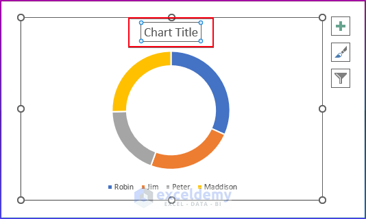
We have added a Chart title named “Sales Information”. Let’s add labels.

Right-click on the chart.
Select Add Data Labels.

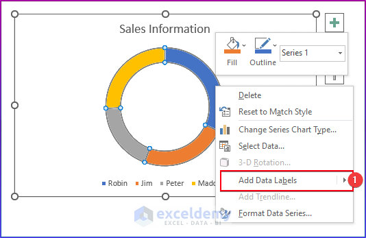
We want to change the color for better visualization.

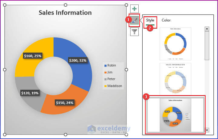
Select the chart.
Click on Chart Styles.
Select a Style. We have selected the marked format in the image below, but you can select any other format you like.

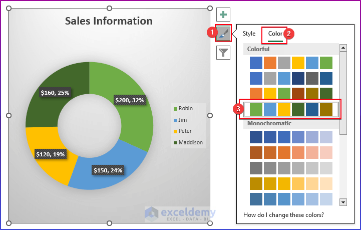
You can also change the color of your doughnut chart.

Select the doughnut chart.
Go to Chart Styles and select Color.
Choose the color palette according to your preference. We have selected a color palette from the image.

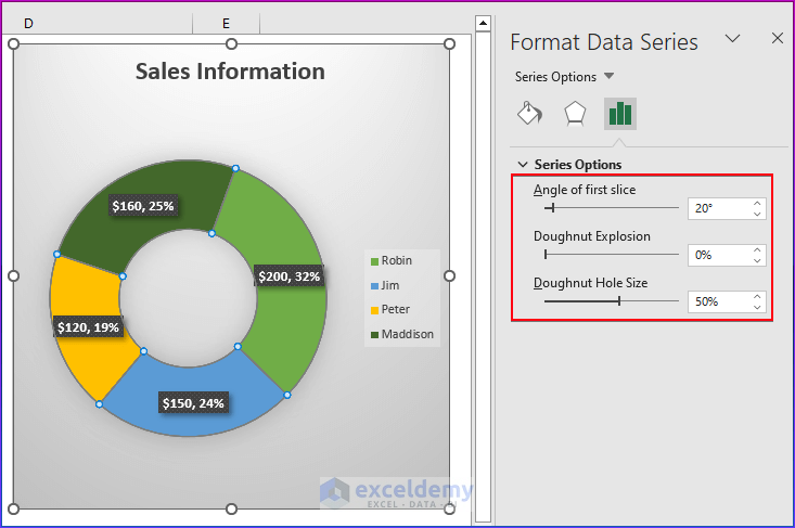
You can modify the doughnut’s thickness and other parameters.

Choose the doughnut chart. The right side of the screen will display the Format Data Series pane.
We have kept it around 20 degrees here.
To alter the doughnut chat’s thickness, alter the size of the doughnut hole. We have kept it at 50%

Here’s the result.

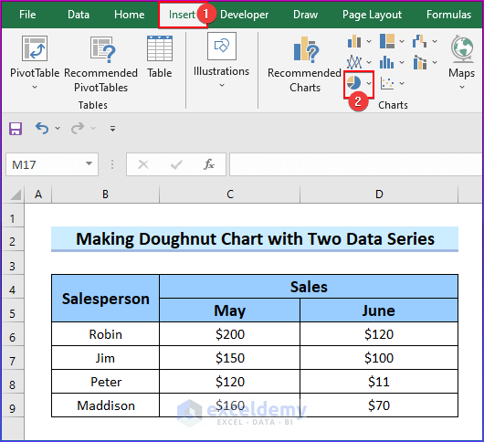
Example 2 – Making a Doughnut Chart with Two Data Series

Go to the Insert tab.
Select Insert Pie or Doughnut Chart from the Charts options.

Click on the Doughnut chart option.

You will see a blank chart.
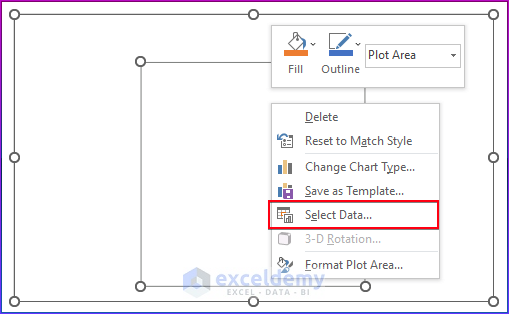
Right-click on the Doughnut chart and choose the Select Data option.

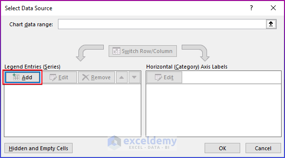
Click on Add.

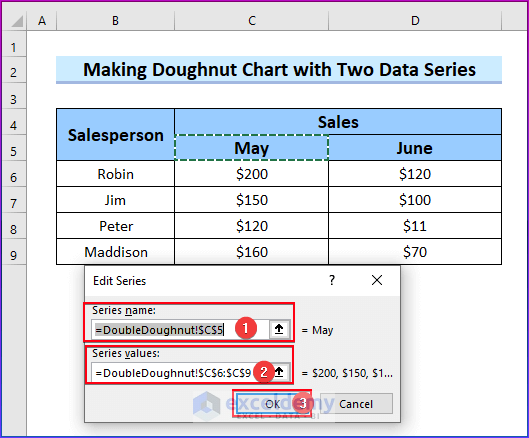
Insert “Series name” as cell C5 and “Series values” from as C6:C9 cells.
Click OK.

Click on Add.

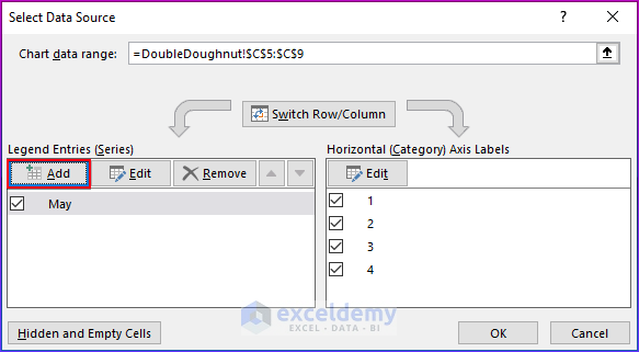
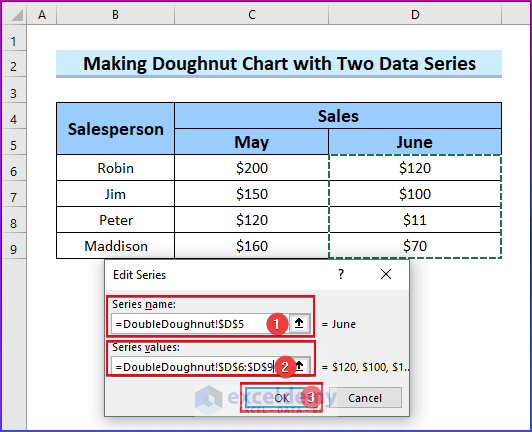
Insert “Series name” as cell D5 and “Series values” as D6:D9 cells.
Click OK.

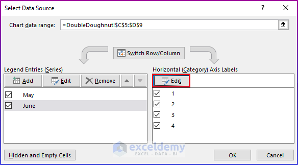
On the right-hand side, choose Edit.

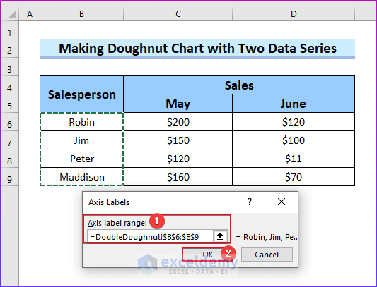
Add the Axis label range as B6:B9 cells.
Click OK.

Click OK.

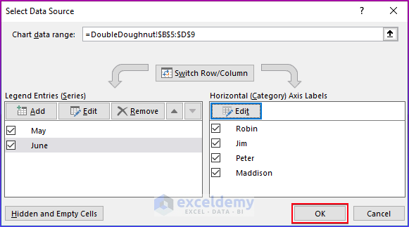
You will get your desired doughnut with two data series values.

How to Create a Doughnut Chart with Multiple Rings in Excel?

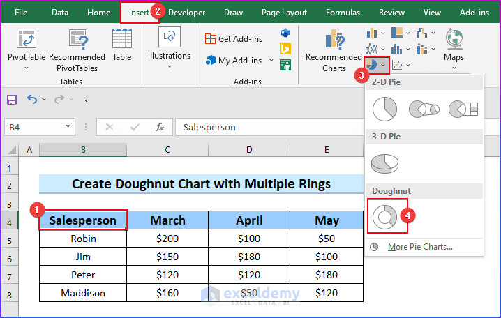
Select the dataset that you want to include in your doughnut chart.
Go to the Insert tab.
Select Insert Pie or Doughnut Chart from the Charts options.
From the drop-down menu, choose Doughnut chart.

You will see a doughnut chart in your worksheet
Change the chart title.

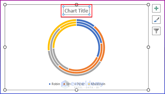
We have added a Chart title named “Sales Information”.
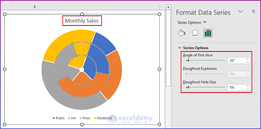
Right-click on any doughnut rings and you will see the Format Data Series window.
Reduce the Doughnut Hole Size according to your preference for getting a better view of the chart.

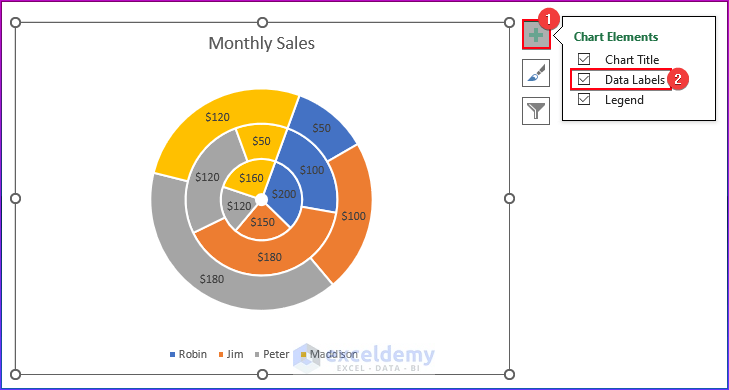
We will add data labels to your doughnut chart.

Click on the chart.
Select the Chart Elements option.
Choose Add Data Labels.

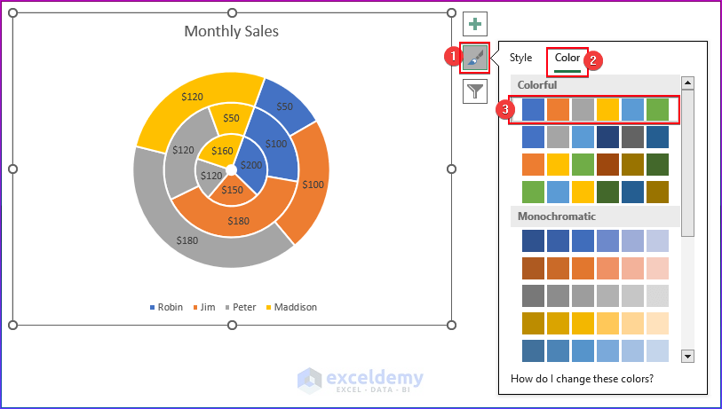
You may also change the doughnut chart’s color as well.

Select the chart.
Navigate to Chart Styles.
Choose Color.
Choose the color scheme based on your personal preferences.

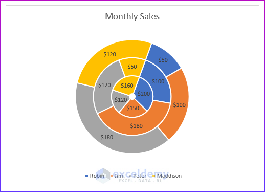
Here’s a sample doughnut chart with multiple rings.

How to Make a Doughnut Chart with the Total in the Middle in Excel?

Select all the data.
Go to the Insert tab.
Click on the Insert Pie or Doughnut Chart option from the ribbon.
Choose the Doughnut chart.

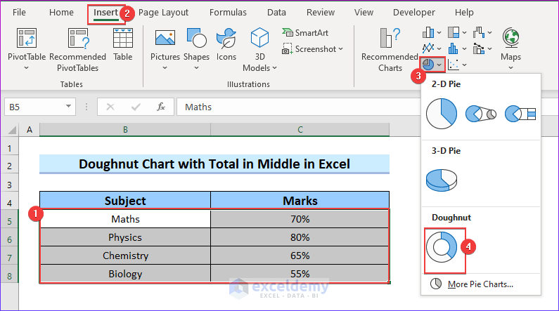
You get a basic donut chart.

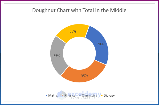
We want to add the total in the middle of the doughnut chart.

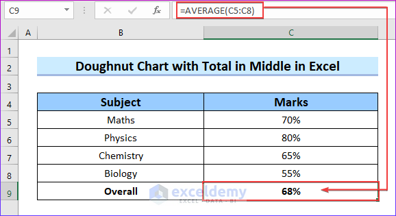
Choose the appropriate value to add in the middle. We want to represent the general average value for my dataset in the center of the doughnut chart.
Insert the following formula in the C9 cell.

=AVERAGE(C5:C8)

Press Enter to get the average value.

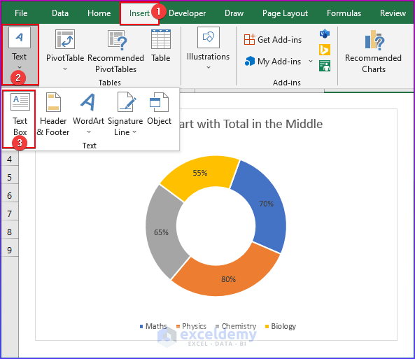
Go to the Insert tab.
From the ribbon, click on the Text option.
Choose Text Box.

Place the Text Box in the center of the doughnut chart.

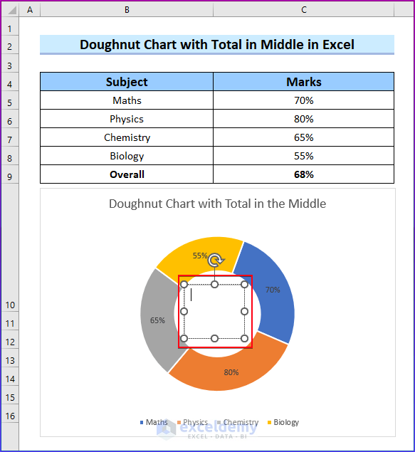
Go to the formula bar.
Use the following formula to represent the value in the middle of the doughnut chart.

=Total_in_Middle!$C$9

Hit Enter.

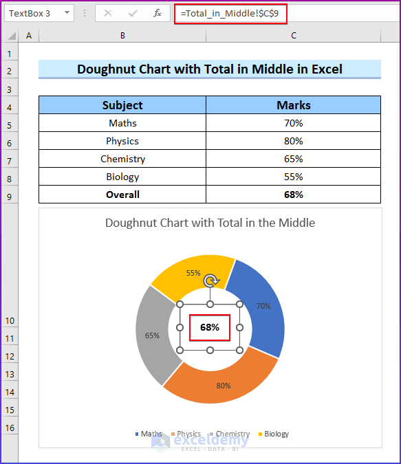
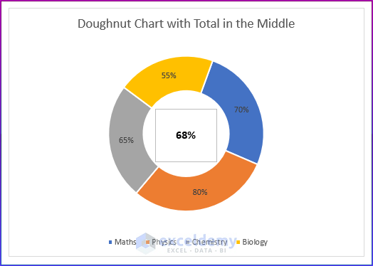
You will get the following output.

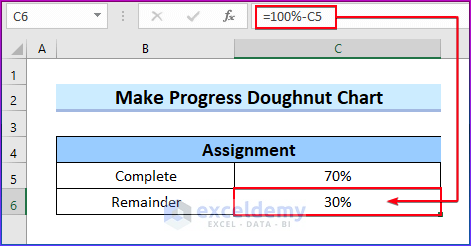
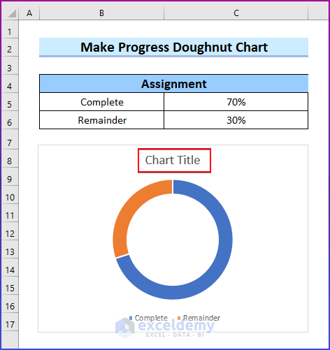
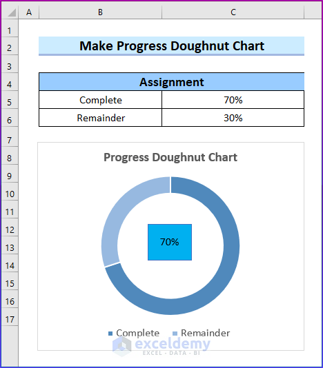
How to Make a Progress Doughnut Chart in Excel?

We have calculated the remaining percentage of the assignment with the following formula in the C6 cell.

=100%-C5

Press Enter.

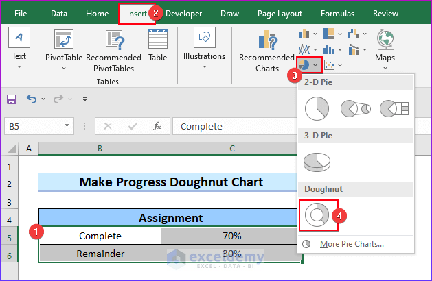
Select the dataset that you want to represent in your doughnut chart.
Go to the Insert tab.
Select Insert Pie or Doughnut Chart from the Charts options.
From the drop-down menu, choose Doughnut chart.

You will see a doughnut chart in your worksheet.
Change the title of the chart.

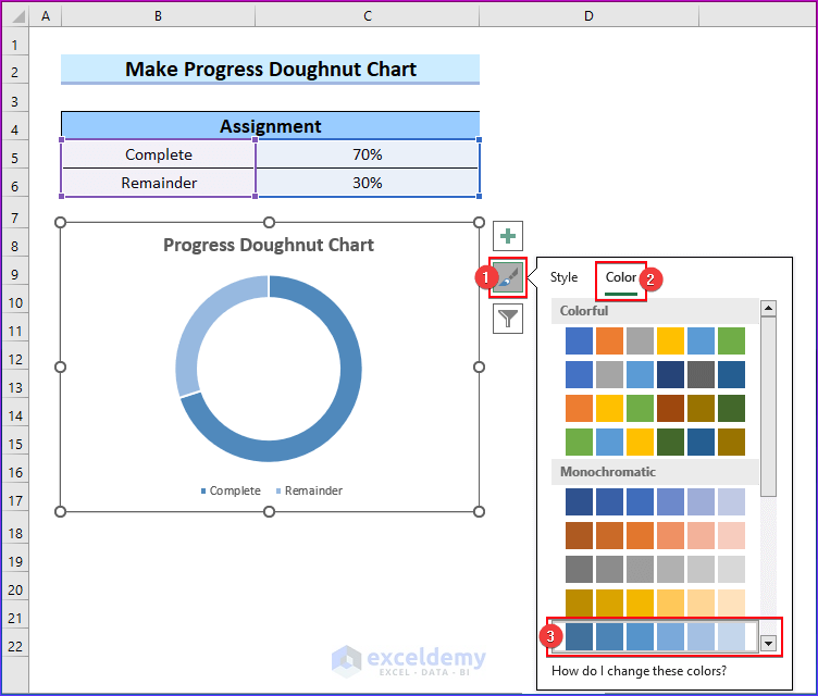
Change the color of your doughnut chart.

Go to the Insert tab.
Click on the Text option.
Choose Text Box.

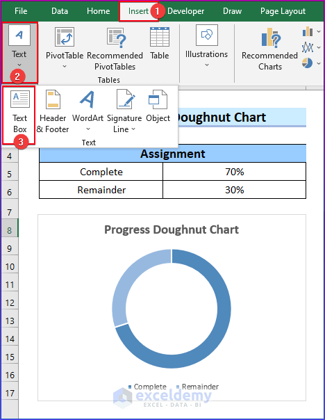
Place the Text Box in the center of the doughnut chart.
Go to the formula bar.
Insert the following formula to represent the progress value in the center of the doughnut chart.

=$C$5

Hit Enter.

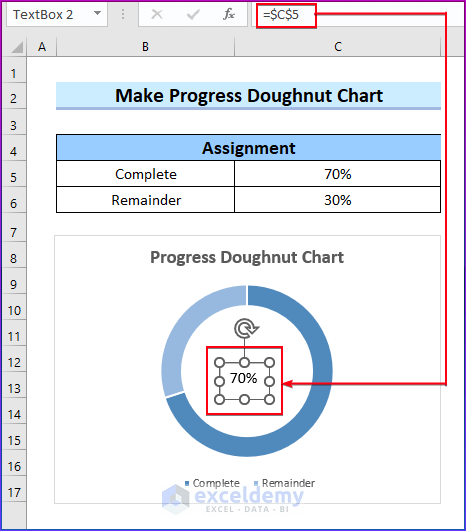
Here’s the result. We modified the textbox a bit.

Things to Remember

To access the modifying tools, you need to select the doughnut chart.
To make a doughnut chart with many rings, you should have a dataset with multiple rows and columns.
Doughnut charts are similar to pie charts and have a central hole.
Doughnut charts are useful when creating visualizations with single, double, or multiple matrices.
Making a chart for 100% matrices is often useful.
There are single-doughnut, double-doughnut, and multiple-doughnut charts available.

Frequently Asked Questions

In Excel, how can I make a Doughnut chart?

To make a doughnut chart in Excel, choose the data for the chart, then go to the Insert tab, click the “Insert Pie or Doughnut Chart” button, and then select the “Doughnut” chart type from the selections.

Can I change the colors of the Doughnut chart segments?

Yes, the colors of the segments in a doughnut chart can be changed. Select the chart, navigate to the Chart Tools Format tab, click the “Shape Fill” or “Shape Outline” button, and select the required color or a custom color scheme.

How can I add labels to the Doughnut chart segments?

To add labels to doughnut chart segments, select the chart, navigate to the Chart Tools Format tab, click the “Data Labels” button, and select the desired labeling option, such as showing the category name, value, or percentage.

In Excel, can I modify the size of the Doughnut chart?

In Excel, you may alter the size of the doughnut chart. Select the chart, then modify the width and height by dragging the scaling handles or entering the exact dimensions in the Format Chart Area box.