Excel Accounting Number Format (Apply and Customize)

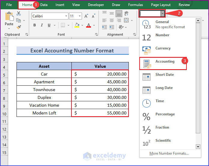
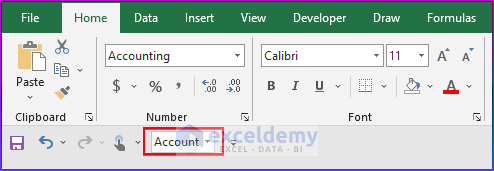
Here’s an overview of where you can find the Accounting format to apply it to cells.

Download the Practice Workbook

What Are the Ways to Apply Accounting Number Format in Excel?

Method 1 – Apply the Accounting Number via the Format Button

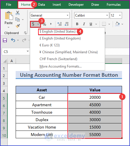
• Select a range of cells you want to format.
• Go to the Home tab.
• Click on the Accounting Number Format button.
• We have chosen the accounting currency “$English (United States)”. If you need to use a different currency, go to the drop-down menu next to the Accounting Number Format button and select the appropriate currency.

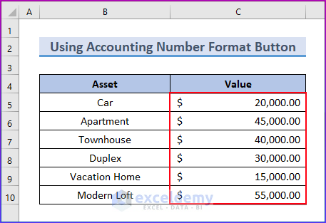
• You will see the output in the following image.

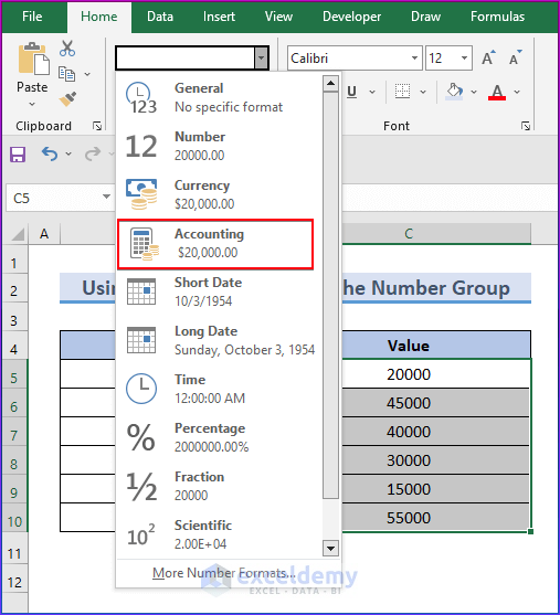
Method 2 – Apply the Accounting Number Format Using the Drop-Down Menu in the Number Group

• Select the range of cells from cell C5 to cell C10.
• Select the drop-down menu button in the Number group on the Home tab.

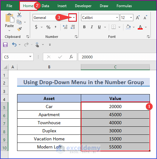
• Select Accounting from the list of formats.

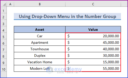
• You will see all the selected cells have been formatted in the below image.

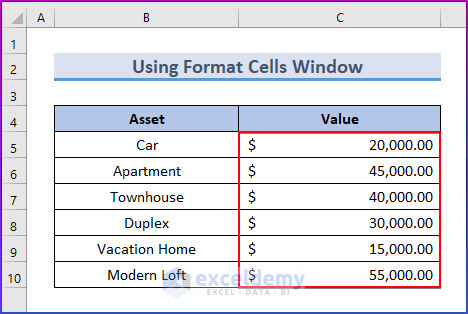
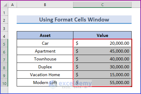
Method 3 – Apply the Accounting Number Format Using the Format Cells Window

• Choose the range of cells to be formatted.
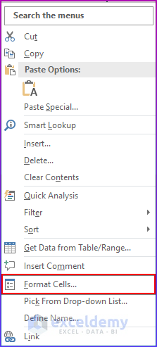
• Right-click on the selection and select Format Cells or press Ctrl + 1 to open the Format Cells window.

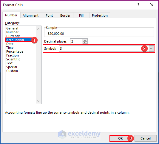
• In the Format Cells window, choose Accounting from the Number tab.
• Select your desired currency format and click OK.

• Here’s the result.

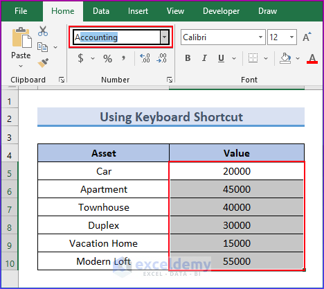
Method 4 – Apply the Accounting Number Format Using a Keyboard Shortcut

• Select the range of cells.
• Press the keys Alt + H + N + A.
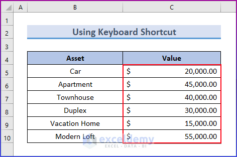
• Press Enter.

• Here’s the result.

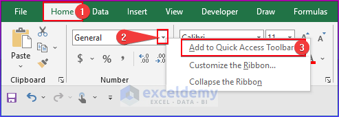
Method 5 – Apply the Accounting Number Format Using the Quick Access Toolbar

• Right-click the drop-down menu button in the Number group on the Home tab.
• Choose the Add to Quick Access Toolbar option.

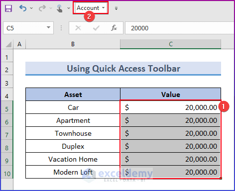
• This will add a little dropdown list to the Quick Access Toolbar area.

• Choose the Accounting format from the Quick Access Toolbar after selecting the range of cells.

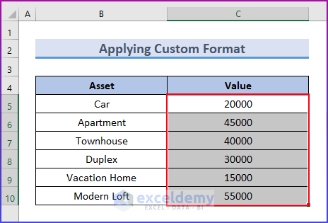
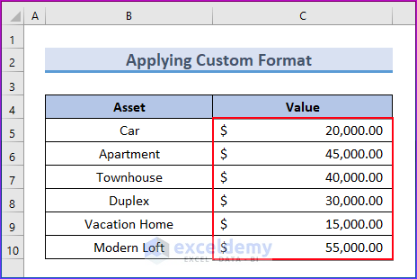
Method 6 – Apply the Custom Format as Accounting Number Format

• Choose the numbers to format.

• To access the Format Cells menu, use the Ctrl + 1 keyboard shortcut.
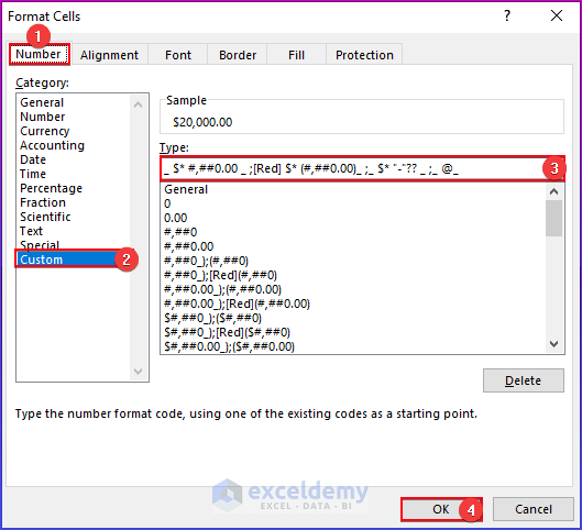
• Navigate to the Number tab.
• In the Category drop-down menu, choose Custom.
• Copy and paste this format string into the Type input.

• Click the OK button.

• Here’s the result.

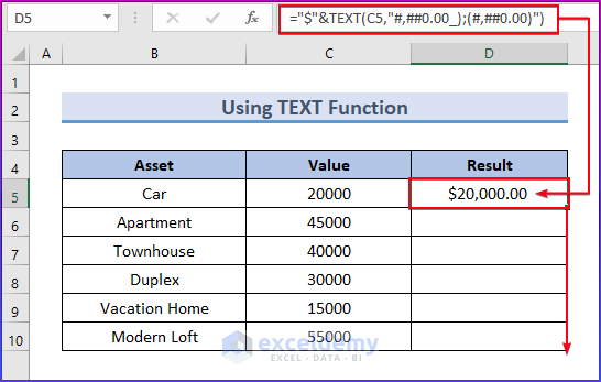
Method 7 – Apply the Accounting Number Format Using the TEXT Function

• Select cell D5 and use the following formula.

• Click Enter.
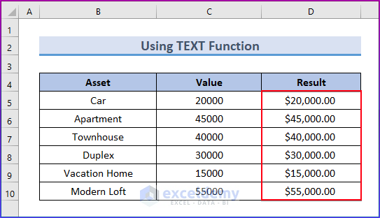
• Drag the Fill Handle icon down to get all the results.

• Here’s the result.

What Are the Ways to Increase/Decrease Decimal Numbers in the Accounting Number Format?

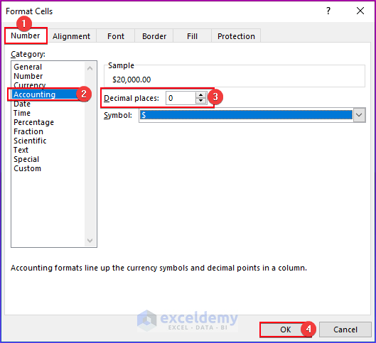
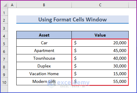
Method 1 – Use the Format Cells Window

• Select the number cells with decimal places.

• Press Ctrl + 1 to open the Format Cells window.
• In the Category drop-down menu, choose the Accounting option under the Number tab.
• Write zero (0) in the Decimal Places option. You can change the value as needed.
• Select the currency symbol if you want.
• Click on the OK button.

• Here’s the result.

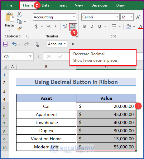
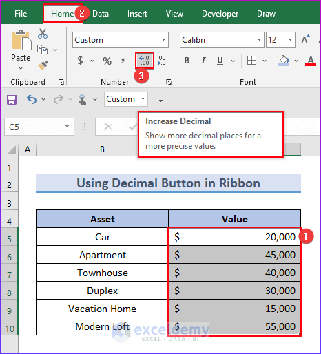
Method 2 – Use the Decimal Button in the Ribbon

• Select the cells.
• Go to the Home tab.
• Choose the Decrease Decimal button from the Number group.
• We will decrease two decimal places to zero (0) decimal places so will click twice on the Decrease Decimal button.

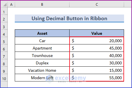
• Here’s the result.

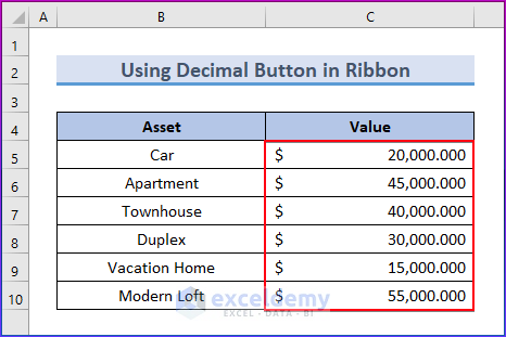
To increase decimal places:

• Click the Increase Decimal button from the Number group under the Home tab.

• We have changed the values from zero decimal places to three decimal places.

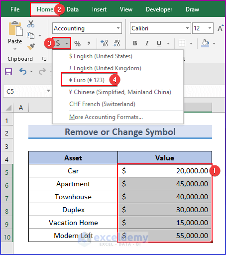
How to Remove or Change Symbols in the Accounting Number Format

• Select the number cells, and all the cells are in Accounting format with United States currency. We will change this format to another currency format.
• Go to the Home tab.
• Click on the Number Format button in the Number group.
• Choose the Euro currency.

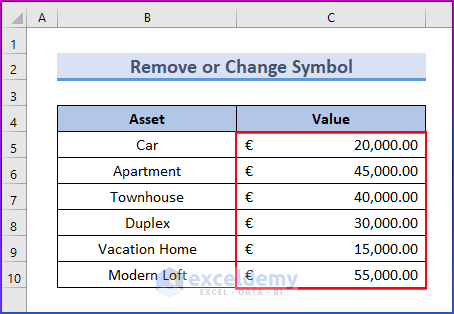
• You will find all the numbers changed to Euro currency in the following image.

Things to Remember

• When inputting values, the user can choose whether or not to include decimal places.
• When you use a custom Excel number format, you change the visual look of a cell’s value without changing the recorded value. When a format is modified, a copy of that format is created; the original format remains unmodified and cannot be erased.
• Custom number formats simply affect how numbers appear in the worksheet; they have no effect on the original numeric value.

Frequently Asked Questions

What are the advantages and disadvantages of Excel’s Accounting Number Format?

The Accounting Number Format in Excel offers benefits such as clear alignment and formatting, increased readability, simple currency symbol insertion, consistent decimal places, and negative number handling.

However, it has some drawbacks, such as restricted customization possibilities, probable calculation concerns, incompatibility with formulas, a lack of globalization, and data analysis difficulties.

What are the differences between Excel Accounting number format and Currency format?

The Accounting Number Format aligns currency symbols and decimal places, uses parentheses for negative numbers, and ensures that all values have consistent decimal places.

The Currency Format, on the other hand, simply adds the currency sign to the numbers without any alignment or special treatment for negative numbers.

Can I use conditional formatting along with the Accounting Number Format?
Yes, you can apply conditional formatting alongside the Accounting Number Format to highlight cells that meet specific criteria. Conditional formatting allows you to visually emphasize certain data based on the rules you define.

Excel Accounting Number Format: Knowledge Hub

<< Go Back to Number Format | Learn Excel