How to Make Negative Accounting Numbers Red in Excel – 3 Methods

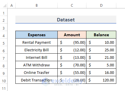
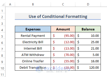
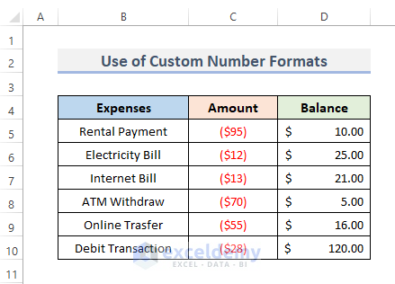
The sample dataset contains monthly expenses, their amount and the balance after the expenses.

Method 1 – Using Excel Conditional Formatting to Make Negative Accounting Numbers Red

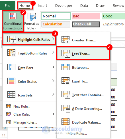
STEPS:

• Select the data cells.
• Go to the Number Format in Number.
• Select Accounting.

• Go to the Home tab.
• In Styles, click Conditional Formatting.
• Select Highlight Cells Rules.
• Select Less Than…

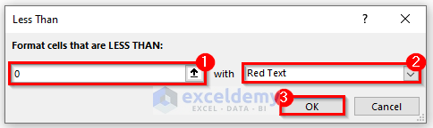
• In the Less Than dialog, enter 0, in Format cells that are LESS THAN.
• In with, select Red Text.
• Click OK.

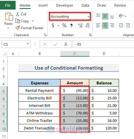
This is the output.

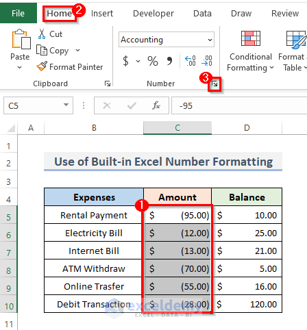
Method 2 – Apply the Built-in Excel Number Formatting To Make Negative Accounting Numbers Red

STEPS:

• Select the data cells.
• Go to the Number Format in Number.
• Select Accounting.
• Go to the Home tab.
• Click the arrow icon in Number or press Ctrl + 1.

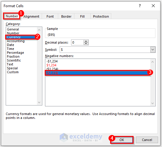
• In the Format Cells dialog box, click Number.
• Choose Currency in Category.
• Select  red color text currency.
• Click OK.

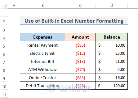
This is the output.

Read More: How to Change Accounting Format in Excel

Method 3 – Using a Custom Number Format to Make Negative Accounting Numbers Red in Excel

STEPS:

• Select the data cells.
• Go to the Number Format in Number.
• Select Accounting.

• Go to the Home tab and choose Number or press Ctrl + 1.
• In the Format Cells dialog box, select Custom in Category.
• Enter the following format in Type.

• Click OK.

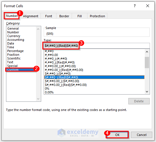
This is the output.

Read More: How to Center Accounting Format in Excel

Download Practice Workbook

Related Articles

• How to Apply Accounting Number Format in Excel
• How to Apply the Accounting Number Format to the Selected Cells in Excel
• How to Simultaneously Apply Accounting Number Format in Excel
• How to Apply Single Accounting Underline Format in Excel
• How to Double Accounting Underline Format in Excel
• [Fixed] Accounting Format in Excel Not Working
• How to Convert Accounting Format to Number Format in Excel

<< Go Back to Accounting Number Format | Number Format | Learn Excel