When you are working with a dataset, and you need to represent some cells as money, then you need them to show as the accounting number format. It generally helps you with the currency information besides the original data. In this article, we will get to know the accounting number format and learn how to apply the accounting number format to the selected cells in Excel with 4 easy methods.
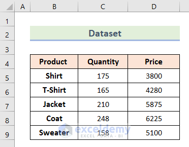
To illustrate, here is a dataset with information on the quantity and price of 5 clothing products. You can see the price cells are showing just as a number. Therefore, we will use 4 easy methods to apply the accounting number format in these cells in Excel.
1. Using Excel Ribbon to Apply Accounting Number Format to Selected Cells
In the first method, we will use Excel ribbon to apply the accounting number format to selected cells. Follow the steps below:
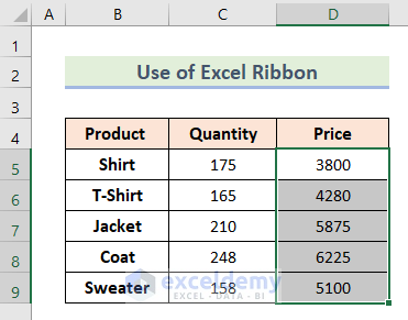
- First, select the cell range D5:D9 that has the price information.
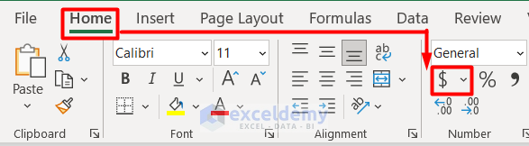
- Secondly, select the Accounting Number Format icon from the Numbers section in the Home tab.
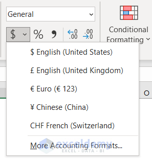
- Then, select the currency you want from the Context Menu.
- Finally, you can see that the price cells are now in the accounting number format.

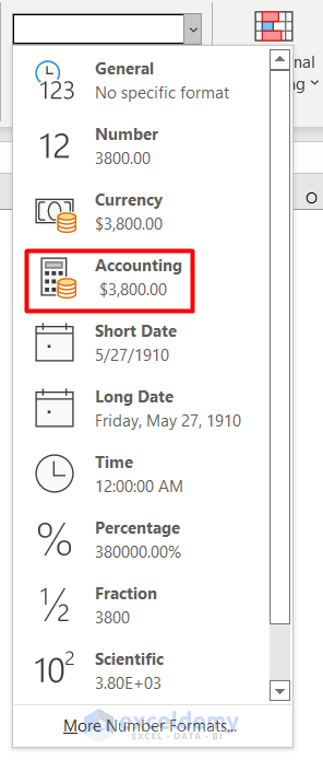
- You can do the same from the Format List in the Number section.
- If you need to change the decimal points, simply click on the Increase Decimal or Decrease Decimal icons in the Number section.

Read More: How to Simultaneously Apply Accounting Number Format in Excel
2. Applying Accounting Number Format to Selected Cells with Format Cells Dialog Box
In the second method, we will learn to apply the accounting number format to selected cells with the format cells dialogue box. Let’s look at the process below:
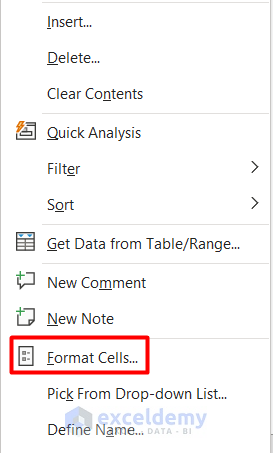
- First, select the cell range D5:D9 and right-click to open the Context Menu.
- Then, select Format Cells.
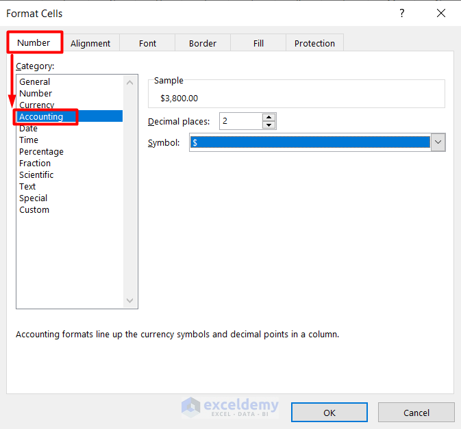
- Therefore, you can see a Format Cells dialogue box pop up.
- Now, go to the Accounting option in the Number section to change Decimal Places and Symbol.
- Press OK.
- You can also get the Format Cells dialogue box in the Numbers section of the Home tab.
- Click on the More Number Formats option in the Format list here.

- That’s it, we have successfully applied the accounting number format in the selected cells.

Read More: [Fixed] Accounting Format in Excel Not Working
3. Using Keyboard Shortcuts to Convert Selected Cells into Accounting Number Format
This one is an easy method. Just follow the simple steps to use keyboard shortcuts to convert selected cells into accounting number format.
- In the beginning, press Alt + H on your keyboard after selecting the cell range D5:D9.
- Then you will get all the shortcuts visible on the Excel ribbon.
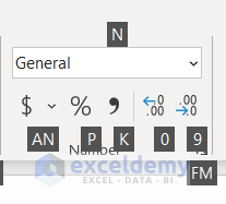
- Now, press Alt + H + AN to open the currency list.
- After that, select the currency you want.

- Finally, you will get your desired output in the selected cells.

4. Inserting Accounting Number Format to Selected Cells with Excel VBA Tool
In this last method, we will insert the accounting number format to selected cells with Excel VBA. Let’s go through the steps below:
- First, select the Visual Basic icon from the Developer tab.
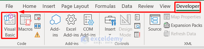
- Following, a new Visual Basic window will appear.
- Here, select Module from the Insert section.
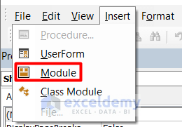
- Now, insert this VBA code into the new blank page.
Sub FormatAccounting()
Dim WkSh As Worksheet
Set WkSh = ThisWorkbook.Sheets(5)
WkSh.Range("D5:D9").NumberFormat = "_($*#,##0.00_);_($*""_""??_);_($*(#,##0.00)_(@_)"
End Sub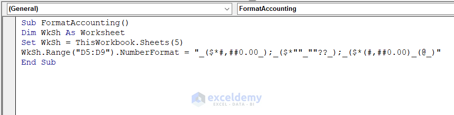
- Finally, you can see that the selected cells are now in the accounting number format.

What Are the Differences Between Accounting Number Format and Currency Format in Excel
Excel users often get confused between the accounting number format and the currency format. Though both of them are number formats with currency information, there are some differences that distinguish them individually. Let’s look at them:
- The accounting number format shows the negative number in parentheses, but the currency format shows it with a minus (–) sign.
- The accounting number format shows the zero (0) as a dash, but the currency format shows it as it is.
- The placement of currency signs and numbers is slightly different from each other.
Things to Remember
- The accounting number format only works with numeric values.
- You cannot remove the thousand separator in the accounting number format.
- If you apply the format in a blank cell, it will automatically convert any number given in the cell afterward to the accounting number format.
Download Practice Workbook
Conclusion
Here, we have learned how to apply the accounting number format to the selected cells in Excel with 4 easy methods. We also tried to make a clear comparison between the accounting number format and the currency format. Hope this was a helpful one. Let us know your suggestions in the comment box.
Related Articles
- How to Apply Accounting Number Format in Excel
- How to Change Accounting Format in Excel
- How to Apply Single Accounting Underline Format in Excel
- How to Apply Double Accounting Underline Format in Excel
- How to Center Accounting Format in Excel
- How to Make Negative Accounting Numbers Red in Excel
- How to Convert Accounting Format to Number Format in Excel
<< Go Back to Accounting Number Format | Number Format | Learn Excel
Get FREE Advanced Excel Exercises with Solutions!
