How to Apply the Accounting Number Format (ANF) in Excel (6 Methods)

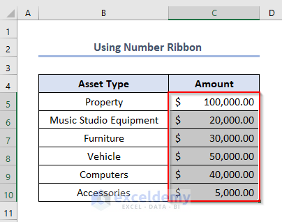
The following image provides a clear overview of the purpose of this Excel tutorial. The right side of the image presents the result of the methods discussed in this tutorial to apply the Accounting Number Format (ANF) in Excel.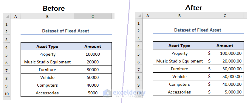

What is Accounting Number Format (ANF)?

The Accounting Number Format (ANF) in Excel is a specific formatting option designed to make numbers and monetary values easier to read for accounting and financial purposes. It includes dollar signs ($), commas for thousands, and parentheses for negative values. This formatting not only prevents errors but also ensures that financial data is interpreted accurately.

Excel offers two main types of number formatting for money and currency-related cell values: Currency format and Accounting Number Format (ANF). While both formats share common features such as showing a currency symbol (usually a “$” sign by default), two decimal points, and comma separators, they have distinct characteristics:

• Currency Format
  • Displays the currency symbol before the number.
  • Right-aligns figures.
  • Allows customization of decimal places.
• Accounting Number Format (ANF)
  • Aligns the currency symbol at the leftmost position for a neat presentation.
  • Uses parentheses for negative numbers.
  • Specifically designed for financial documents, offering a standardized and professional appearance.

Both formats are suitable for financial presentations in Excel, but the Accounting format provides additional features tailored to accounting and financial statements. Your choice between the two depends on the specific requirements of your data presentation and the visual style you aim to achieve.

Understanding the Methods

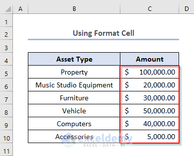
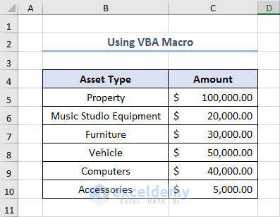
To illustrate the diverse approaches, let’s consider a sample dataset called Fixed Asset. This dataset includes two simple columns with headers: Asset Type and Amount. Our focus in this article is to apply the Accounting Number Format to the Amount column.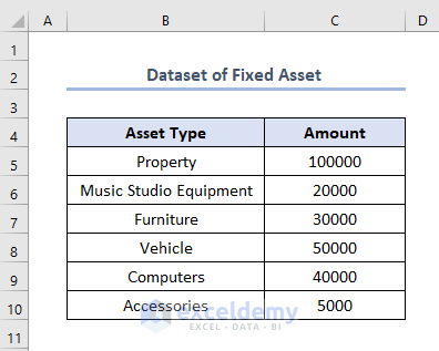

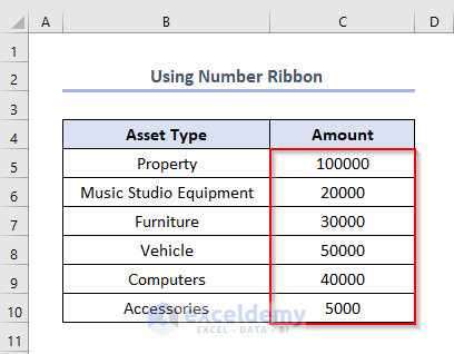
Method 1 – Using Number Group

To quickly apply the Accounting Number Format to your selected data in Excel, follow these steps using the Number Group on the Home tab:

• Select the cells or range of cells you want to format (e.g., C5:C10).
  
• Go to the Home tab in the Excel ribbon.
• Click on the Accounting Number Format symbol ($) within the Number group.

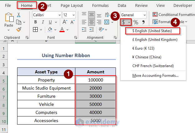
These steps will convert the formats of the selected cells into the Accounting Number Format (ANF), making them suitable for displaying financial data in a clear and organized manner.

Method 2 – Using Number Format Dropdown

The Number Format dropdown menu provides an easy way to apply various number formats, including the Accounting number format, to your data in Excel:

• Select the cells or range of cells you want to format (e.g., C5:C10).
• Go to the Home tab in the Excel ribbon.
• Find the Number Format dropdown.
• Select Accounting from the category list.

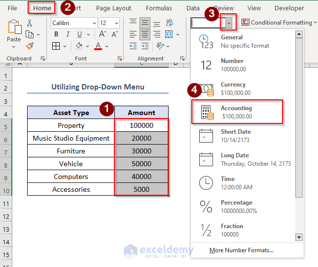
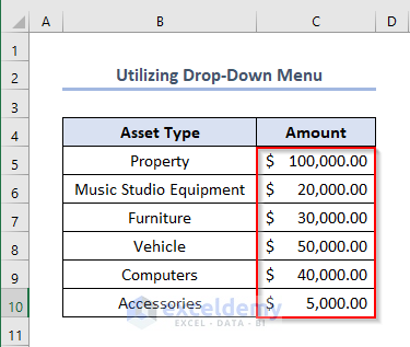
This will change the formats of the selected cells into the Accounting Number Format (ANF), making them suitable to display as financial data.

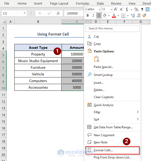
Method 3 – Using Format Cells Dialog Box

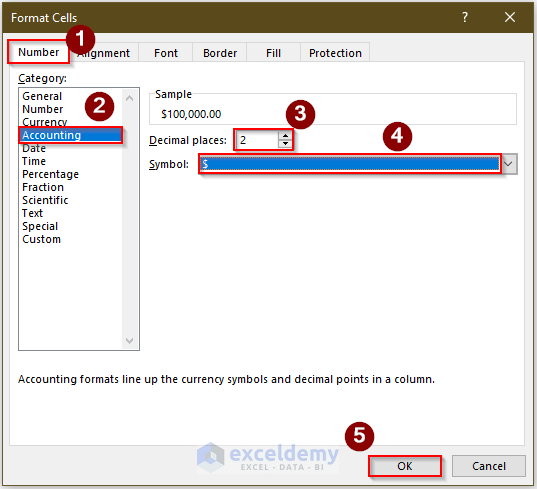
The Format Cells dialog box in Excel allows you to customize formatting options, including the Accounting Number Format:

• Select the cells you want to format (e.g., C5:C10).
• Right-click on the selected cells and choose Format Cells.
  • Shortcut: Press CTRL + 1 to directly open the Format Cells dialog box.

• In the Format Cells dialog box:
  • Click on the “Number” tab.
  • Select “Accounting” from the Category list.
  • Customize the number of decimal places and the symbol field if needed.
• Click OK to apply your number formatting.
  

The above steps will convert the cell formats of the selected cells into Accounting Number Format (ANF), making them suitable to display as financial data in a clear and organized manner.

The Format Cells dialog box is particularly useful when you need detailed adjustments beyond the standard formatting options available in the ribbon or drop-down menus.

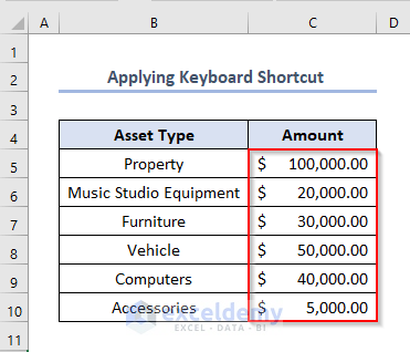
Method 4 – Using Keyboard Shortcuts

While there isn’t a dedicated keyboard shortcut for applying the Accounting Number Format (ANF) in Excel, you can use the following keyboard shortcuts to activate the Accounting Number Format button ($) on the Home tab of the ribbon:

• Select the cells you want to format (e.g., C5:C10).
• Press ALT + H + A + N on the keyboard.
• The most used currency list will pop up.
  
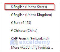
• Press ENTER after confirming your currency choice.

The cell formats of the selected cells will be converted into Accounting Number Format (ANF).

Note: The ALT + H + A + N shortcut changes the currency format for the selected cells when the Home tab is activated. Be cautious not to confuse it with other shortcuts that open different tabs or align cell values.

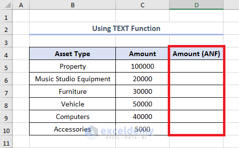
Method 5 – Using TEXT Function

To apply the Accounting Number Format (ANF) in Excel using the TEXT function, follow these steps:

• Insert a New Column:
  • Add a new column where you want to apply the Accounting Number Format. Let’s call this column Amount (ANF).

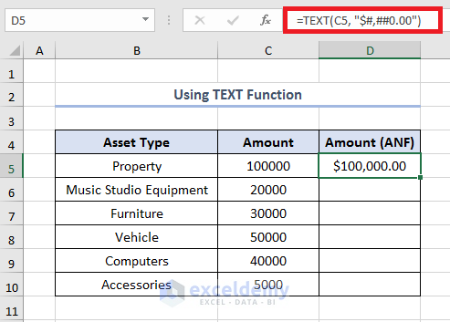
• Select the First Cell:
  • Choose the first cell in the Amount (ANF) column where you want to apply the Accounting Number Format. For example, if your data starts in cell D5, select that cell.

• Enter the Formula:
  • Insert the following formula into the selected cell:

=TEXT(C5, "$#,##0.00")
(Replace C5 with the appropriate cell reference based on your dataset.)

• • Press Enter to apply the formula.

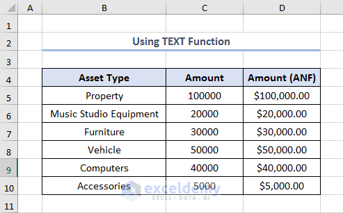
• Fill Down:
  • Click and drag the Fill Handle (the small square at the bottom-right corner of the selected cell) down to apply the formula to the entire column.

These steps will change the formats of the selected cells into the Accounting Number Format (ANF), making them suitable to display as financial data in a clear and organized manner.

Method 6 – Using a VBA Macro

To apply the Accounting Number Format (ANF) in Excel using a VBA macro, follow these instructions:

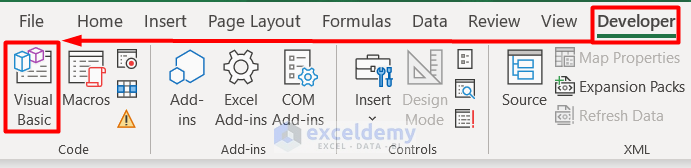
• Open the VBA Editor:
  • Click on the Visual Basic tool from the Developer tab.
    • Shortcut: Press Alt + F11 to open the VBA editor directly.

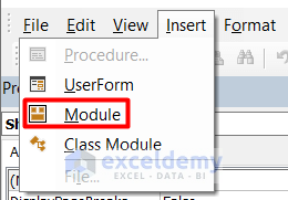
• Insert a New Module:
  • Go to Insert and select Module or right-click on any item in the project explorer on the left and select Insert and click on Module.

  

• Copy and Paste the Code:
  • Copy and paste the following code into the module:

  Sub ApplyAccountingNumberFormatToColumn()
  
  Dim ws As Worksheet
  Dim rng As Range
  Dim lastRow As Long
  
  ' Set the worksheet
  Set ws = ThisWorkbook.Sheets("Using VBA Macro")
  ' Change "Using VBA Macro" to your sheet name
  
  ' Set the range to the entire column A
  Set rng = ws.Range("C5:C10")
  
  ' Apply Accounting Number Format to the range
  rng.NumberFormat = "_($* #,##0.00_);_($* (#,##0.00);_($* "" - ""??_);_(@_)"
  
  End Sub

• Close the VBA Editor:
  • Save your changes and close the VBA editor.

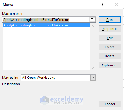
• Run the Macro:
  • Press Alt + F8 to open the Macro dialog box.
  • Select ApplyAccountingNumberFormatToColumn from the list.
  • Click Run.
    • Shortcut: You can also press F5 to run the macro.

The above steps will convert the cell formats of the specified range (C5:C10) into the Accounting Number Format (ANF), making them suitable for displaying financial data.

How to Apply Accounting Number Format with No Decimal Places

The default application of the Accounting Number Format (ANF) in Excel automatically adds two decimal places to numbers. However, if you want to remove decimal places from your formatted data, follow these steps:

• Select the cells you want to format.
• Right-click on the selected cells.
• From the context menu, choose Format Cells.
• The Format Cells dialog box will appear.
• Go to the Number tab.
• Select Accounting from the Category list.
• In the dialog box, set the Decimal places field to 0.
• Alternatively, you can choose any other desired number of decimal places and currency symbols.

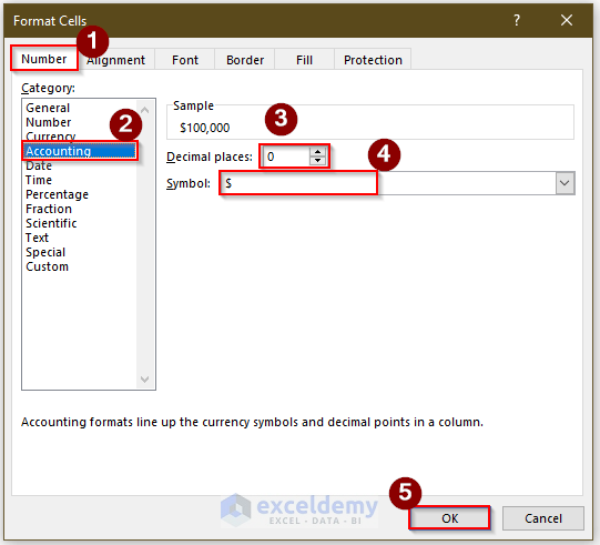
• Click OK to apply the Accounting number format with no decimal places to the selected cells.

This manual process allows you to customize the Accounting number format according to your specific requirements.

How to Customize the Application of Accounting Number Format (ANF) to Meet Your Requirements

The Accounting Number Format (ANF) in Excel can be further customized to match specific user preferences. To do this:

• Select Custom Format:
  • In the Format Cells dialog box, choose Custom from the Category list.

• Enter or Select a Format Code:
  • In the Type field, you can either select from existing format codes or enter your own.
  • The format code determines how cell contents will be displayed.

• Common Format Codes:
  • Common format codes for ANF include adding currency symbols, adjusting decimal places, and handling negative numbers.

In Accounting Number Format (ANF), you typically employ various codes to format numbers. These may involve incorporating currency symbols, determining decimal places, and formatting negative numbers. For instance, to represent negative numbers within parentheses, you can utilize the format code: “($#,##0.00);($#,##0.00)”. Additionally, conditional formatting allows for the application of different ANF styles based on specific conditions, like highlighting cells with negative values in red. By tailoring ANF settings in Excel, you can effectively present your financial information in a clear and polished manner.

Download Practice Workbook

You can download the practice workbook from here:

Frequently Asked Questions

• How to Apply Accounting Number Format to Selected Cells:
  • From the perspective of this article, using the Format Cells dialog box is a practical way to apply the Accounting Number Format to selected cells:
    1. Select the specific cells (hold the CTRL key to select multiple cells).
    2. Right-click on any of the selected cells.
    3. Choose Format Cells.
    4. In the Format Cells dialog box, go to the Number tab.
    5. Select Accounting from the Category list.
    6. Customize your requirements (e.g., decimal places, currency symbol).
    7. Click OK.
  • Alternatively, you can use the Accounting format button (as mentioned in previous examples).

• How to Simultaneously Apply Accounting Number Format in Excel:
  • To apply the Accounting Number Format to multiple cells or a range:
    1. Select the specific cells (hold the CTRL key to select multiple cells).
    2. Right-click on any of the selected cells.
    3. Choose Format Cells.
    4. Follow the same steps as above to select Accounting and customize your requirements.
  • Consider adding the Accounting format button to the Quick Access Toolbar for quicker access.

• Fixing Negative Numbers in Parentheses:
  • Excel allows flexibility in displaying negative numbers within parentheses or with a minus sign.
  • To remove parentheses from negative numbers:
    • Select Custom from the Category list in the Format Cells dialog box.
    • Use the format code: ($* #,##0.00_);$* "-"#,##0.00; $* "-"??_);_(@_)
    • This code displays negative numbers without parentheses and with a minus sign.

• Adding the Accounting Format Button to Quick Access Toolbar:
  • Right-click on the Accounting format button in the Home tab.
  • Choose Add to Quick Access Toolbar.
  • This provides quick access to the formatting option without navigating through multiple steps.

• Clearing Accounting Number Format in Excel:
  • To remove Accounting Number Format from selected cells:
    • Select the cell or range of cells.
    • Click on the Home tab > Styles group > Clear button.
    • Choose Clear Formats from the drop-down menu.

<< Go Back to Accounting Number Format | Number Format | Learn Excel