This article illustrates how to apply accounting number format in Excel simultaneously. This is a very widely used number formatting in Excel. Unlike the currency format, it aligns the currency signs ($) column-wise and shows negative numbers inside brackets. If you work with currency or sales, then you will often need to apply the accounting number formatting to multiple ranges simultaneously. Follow the article to learn how to easily do that in Excel.
How to Apply Accounting Number Format Simultaneously in Excel: Step-by-Step
Follow the steps below to be able to apply the accounting number format simultaneously in Excel.
📌 Step 1: Organize Data
- Assume you have the following dataset. Here, you need the Sales and Amount columns to be formatted in the accounting number format. The following steps will enable you to do that.

Read More: What Is Accounting Number Format in Excel
📌 Step 2: Select Data & Apply Formatting
- First, select the range C5:C10. Then click on the $ sign in the Number group from the Home tab.

- After that, you will see the following result. You can choose a different currency from the dropdown arrow beside the $ sign.
- Now you can select the range E5:E10 and repeat the same procedure to get a similar result.

Read More: How to Center Accounting Format in Excel
📌 Step 3: Select Multiple Ranges
- Alternatively, you can apply the accounting number format to both columns simultaneously by selecting them first. Select range C5:C10, hold the CTRL key and then select the range E5:E10. This way, you will be able to select both columns.

Read More:How to Apply the Accounting Number Format to the Selected Cells in Excel
📌 Step 4: Apply Accounting Number Format
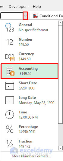
- Now, click on the dropdown arrow beside the General number format in the Number group from the Home Next, choose the Accounting number format.
- Alternatively, you can click on More Number Formats or press CTRL+1 to open the Format Cells dialog box.
- Then, select the Accounting category from the Number tab. Next, fix the decimal places as required and choose the proper currency. Finally, click OK.

- After that, you will see the following result. You can also use the ALT+H+AN+Enter shortcut for that.

Read More: [Fixed] Accounting Format in Excel Not Working
Things to Remember
- You need to hold CTRL to select multiple ranges to apply the accounting number format simultaneously to them.
- You can format the data ranges in accounting number format even before entering any data. This way, whenever you enter the numbers, they will be formatted automatically.
Download Practice Workbook
You can download the practice workbook from the download button below.
Conclusion
Now you know how to apply accounting number format simultaneously in Excel. Do you have any further queries or suggestions? Please let us know using the comment section below.
Related Articles
- How to Apply Double Accounting Underline Format in Excel
- How to Apply Single Accounting Underline Format in Excel
- How to Convert Accounting Format to Number Format in Excel
- How to Make Negative Accounting Numbers Red in Excel
- How to Change Accounting Format in Excel
<< Go Back to Accounting Number Format | Number Format | Learn Excel
Get FREE Advanced Excel Exercises with Solutions!
