Negative Number in Excel (Add, Format, and Convert)

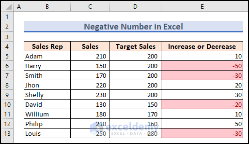
Here’s an overview of negative numbers in Excel and how they can be formatted.

Download the Practice Workbook

Why Do We Use Negative Numbers in Excel?

• Presenting losses or expenses: Negative numbers are commonly used to indicate financial losses, expenses, or deductions. They allow for accurate tracking and calculation of negative values, such as costs, liabilities, or reductions in value.
• Expressing opposite values: Negative numbers represent the opposite of positive numbers, indicating a decrease or opposite change.
• Analyzing deviations: Negative numbers analyze variations from expected values, aiding performance analysis and decision-making.
• Representing budget reports: In budget reports, negative values highlight negative budgets and areas of overspending.
• Cash flow management: Negative numbers are crucial for managing cash flow in Excel. They represent cash outflows, expenses, or debts, enabling accurate tracking and forecasting of financial inflows and outflows.
• Mathematical operations: Negative numbers are essential for math operations, allowing subtraction and expression of decrease or reduction.

How to Show Negative Numbers in Excel

Method 1 – Using the Custom Format Feature

• Select the data range.
• Press Ctrl + 1.

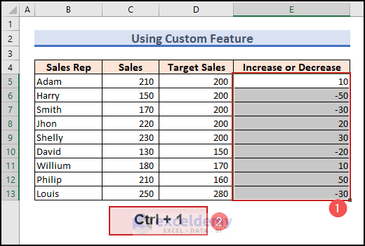
• A Format Cells window pops up.
• Choose Number tab.
• Select a Custom feature from the Category drop-down list.
• Select the following format from the Type drop-down list and hit OK.

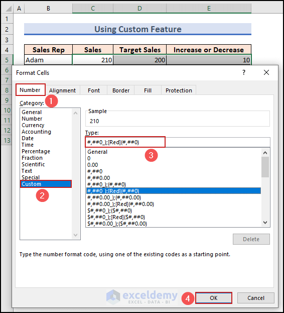
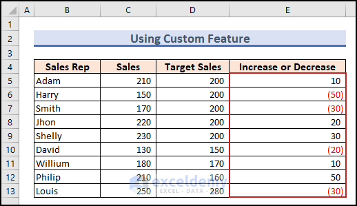
• This shows negative numbers in red.

Method 2 – Applying an Inbuilt Number or Currency Formatting

• Select your data range.
• Go to the Home tab and choose the Number Format dialog launcher from the Number group or press Ctrl + 1.
• Choose the Number tab.
• Select Number from the Category drop-down list.
• Choose a negative number and press OK.

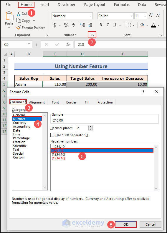
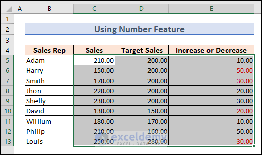
• Here is the final output showing negative numbers.

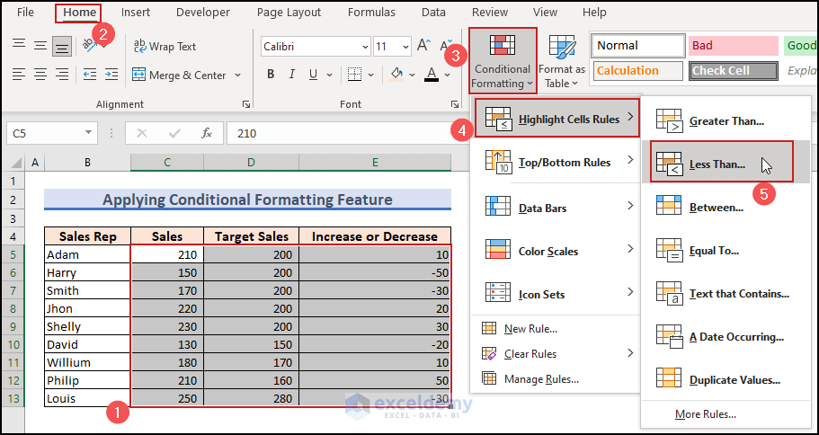
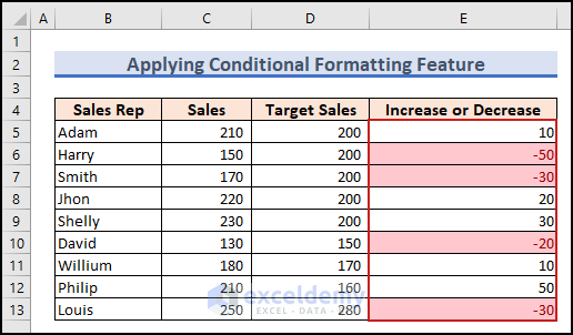
Method 3 – Using Conditional Formatting

• Select the data range.
• Go to the Home tab and Styles group, then select Conditional Formatting, choose Highlight Cells Rules, and pick Less Than.

• A Less Than dialog box will appear.
• Insert 0 in the box on the left and choose the Light Red Fill with Dark Red Text format to the right.
• Hit OK.

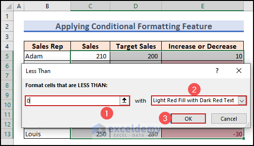
This highlights the negative numbers using the Conditional Formatting feature.

Method 4 – Run an Excel VBA Code

• Press Alt + F11 to pop up the Microsoft Visual Basic Applications window.
• Select Module from the Insert tab to open a Module for inserting the VBA code.
• Paste the below VBA code in that Module.

Sub Show_Negative_Numbers()
Dim ma_rng As Range
For Each ma_rng In Selection
	If ma_rng.Value < 0 Then
    	ma_rng.Font.Color = vbRed
	Else
    	ma_rng.Font.Color = vbBlack
	End If
Next ma_rng
End Sub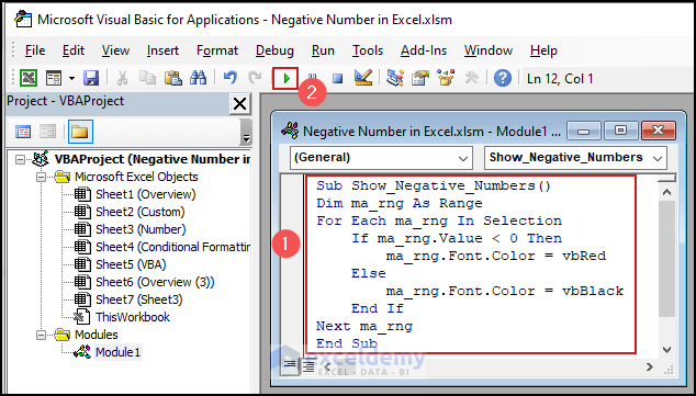

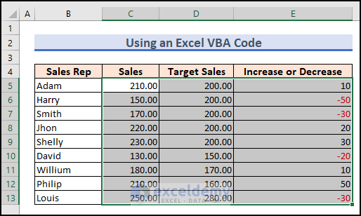
• After running the Macro, you will see the negative numbers in the Red color font.

Read More: Excel Formula to Return Zero If Negative Value is Found

How to Add Negative Numbers Using the SUMIF Function in Excel

• Insert the following SUMIF function in cell C11 to add negative numbers in Excel.

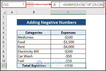
How to Convert Negative Numbers to Positive Using the ABS Function in Excel

• Use the ABS function in cell F5 to convert the negative values to positive and AutoFill the formula.

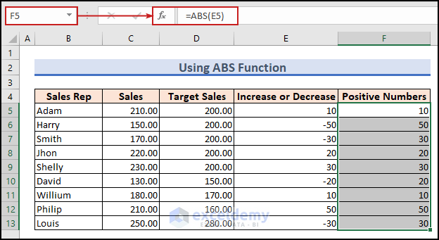
How to Convert Positive Numbers to Negative in Excel

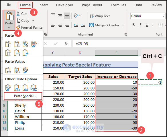
Method 1 – Applying the Paste Special Feature

• Type -1 in any cell and press Ctrl + C.
• Select cells E5 to E13.
• Go to the Home tab.
• Choose the Paste Special feature from the Clipboard group.

• Select the Multiply option under the Operation group.
• Press OK.

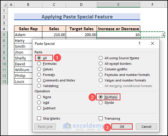
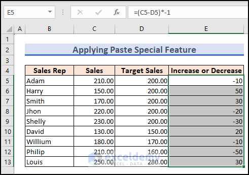
• This converts positive numbers to negative numbers.

Method 2 – Using the IF Function

• In cell F5, insert the following formula and Autofill it.

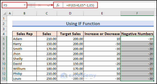
How to Make All Negative Numbers Zero in Excel

• Enter the following formula in cell F5 and autofill it.

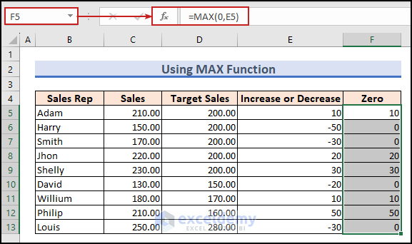
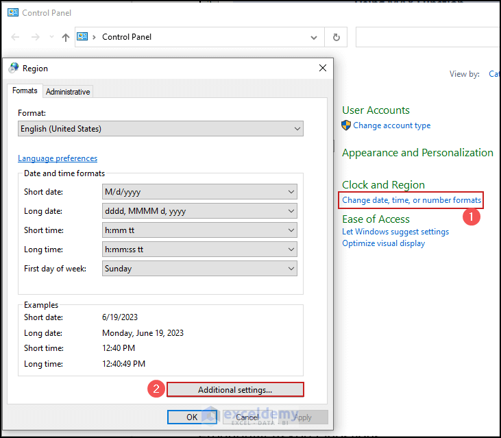
What to Do When Negative Numbers Aren’t Showing with Parentheses in Excel+

• Open the Control Panel.
• Choose Change date, time, or number formats.
• The Region window will pop up.
• Select Additional settings…

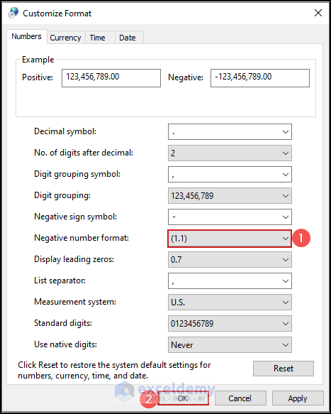
• From the Customize Format window, select the format (1.1) for the Negative number format.
• Click OK.

• Close the Excel file and reopen it.

Things to Remember

• When using the Paste Special method, make sure to copy (-1) and select the range after that. Otherwise, you won’t get the desired result.
• If you have used the VBA code, make sure to save the file as the Enabled Macro book. Otherwise, the code won’t run.

Frequently Asked Questions

Why is Excel unable to sum the negative numbers?

Excel is unable to sum negative numbers by default because the SUM function treats negative numbers as subtracting from the total rather than adding to it. This is designed to align with traditional mathematical conventions where negative numbers represent deductions or debts. However, you can still calculate the sum of negative numbers in Excel by using alternative formulas or adjusting the settings.

How can I perform calculations with negative numbers in Excel?

Excel treats negative numbers like any other numbers when performing calculations. You can use mathematical operators such as addition (+), subtraction (-), multiplication (*), and division (/) with negative numbers just as you would with positive numbers.

Can negative numbers be used in conditional formatting?

Yes, negative numbers can be used in conditional formatting to apply specific formatting styles based on their values. This allows you to highlight or emphasize negative numbers in your Excel worksheets.

Negative Number in Excel: Knowledge Hub

<< Go Back to Number Format | Learn Excel