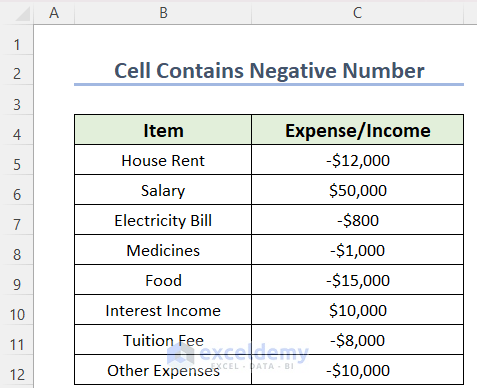
The following dataset showcases Item, and Expense/Income.
Example 1 – Use the COUNTIF Function If the Cell Contains a Negative Number
Steps:
- Select a cell to see the result, here C14.
- Use the following formula in C14.
=COUNTIF(C5:C12,"<0")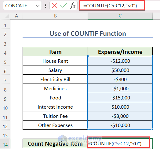
Formula Breakdown
The COUNTIF function counts cells which fulfill the given condition.
- C5:C12 is the data range.
- “<0” is the criteria.
- Press ENTER.
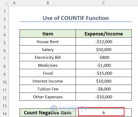
This is the output.
Read More: Excel Formula to Return Zero If Negative Value is Found
Example 2 – Using the SUMPRODUCT Formula
Steps:
- Select a cell to see the result, here C14.
- Use the following formula in C14.
=SUMPRODUCT(--(C5:C12<0))- Press ENTER.
This is the output.
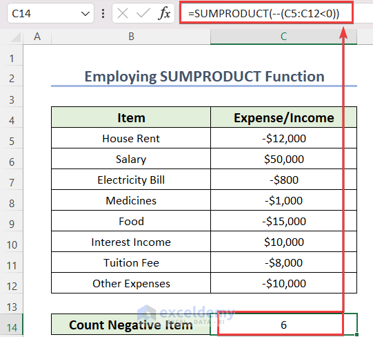
Formula Breakdown
The SUMPRODUCT function will return the sum of the array which fulfills the criteria.
- C5:C12<0 is the criteria. These criteria go through each cell of C5:C12 and check whether the cell value is less than 0. If the cell value is less than 0, it will return TRUE. Otherwise, FALSE.
- Output: {TRUE,FALSE,TRUE,TRUE,TRUE,FALSE,TRUE,TRUE}.
- –(C5:C12<0) converts the output into Boolean terms.
- Output: {1,0,1,1,1,0,1,1}.
- SUMPRODUCT returns the summation of the above output.
- Output: 6.
Read More: Excel Formula to Return Blank If Cell Value Is Negative
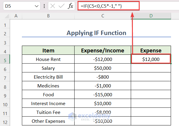
Example 3 – Applying the IF Function If a Cell Contains a Negative Number
Steps:
- Select a cell to see the result, here D5.
- Use the following formula in D5.
=IF(C5<0,C5*-1," ")- Press ENTER.
Formula Breakdown
The IF function performs a logical test.
- C5<0 is the logical test. It checks whether the value of C5 is less than 0.
- C5*-1 —> if the value is less than 0, the cell value is multiplied by -1.
- ” ” —> if the logic fails, a blank space is returned.
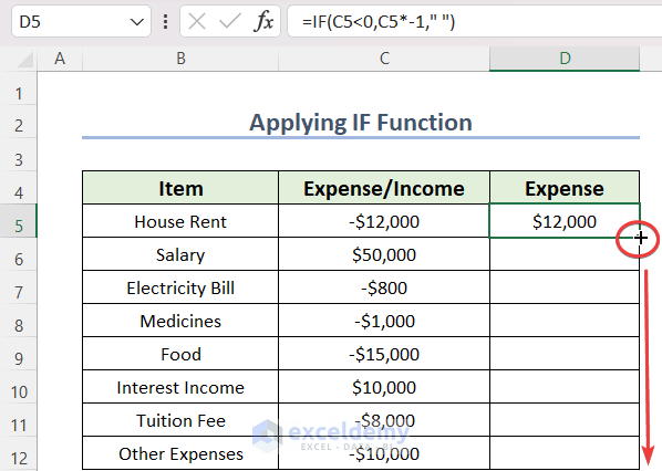
- Drag down the Fill Handle to AutoFill the rest of the cells.
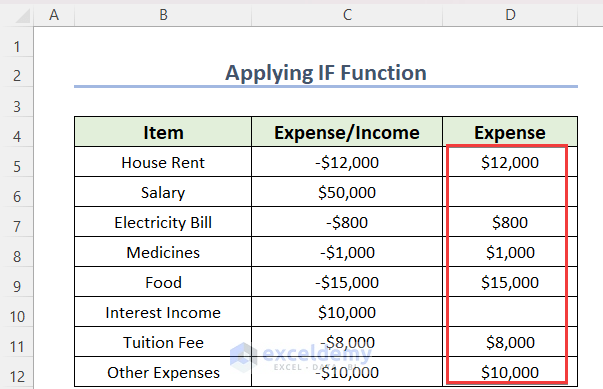
This is the output.
Read More: How to Put a Negative Number in Excel Formula
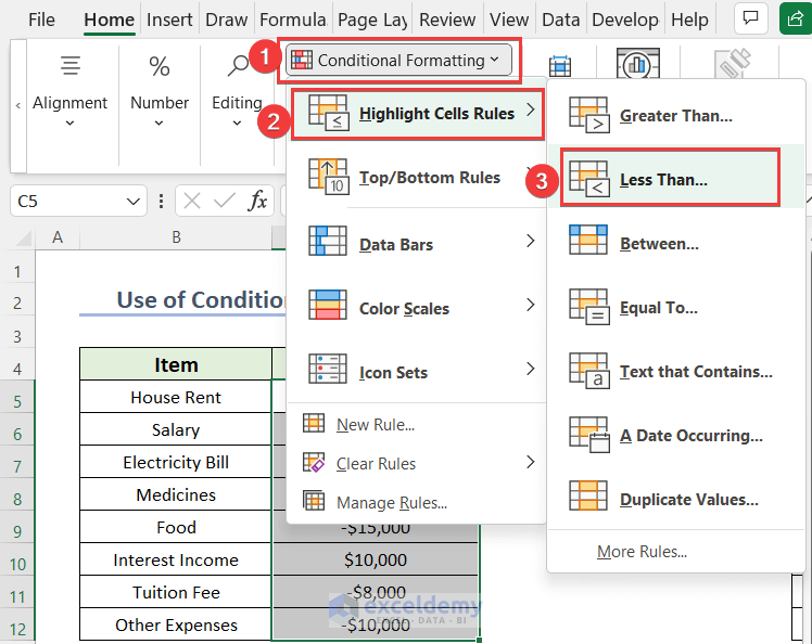
Example 4 – Using the Conditional Formatting Feature
- Select C5:C12.
- Go to the Home tab.
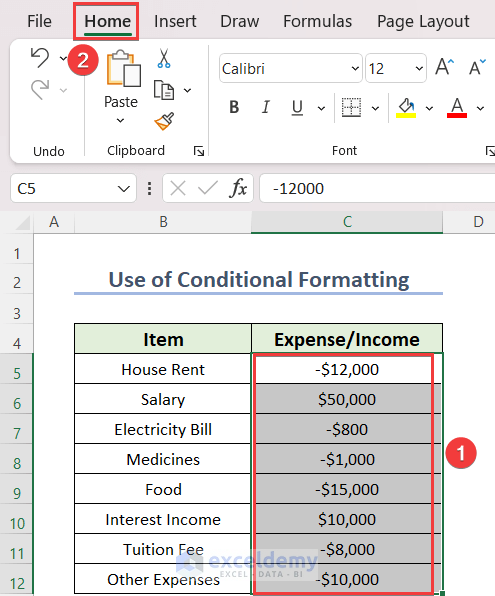
- Select Conditional Formatting.
- In Highlight Cells Rule, choose Less Than… .
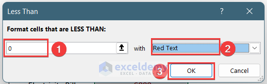
In the Less Than dialog box:
- Enter 0 in Format cells that are LESS THAN.
- Select a color. Here, Red Text.
- Click OK.
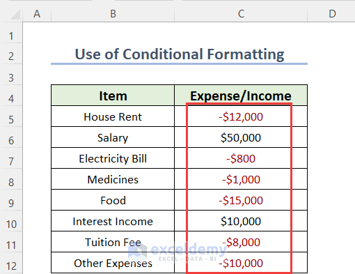
This is the output.
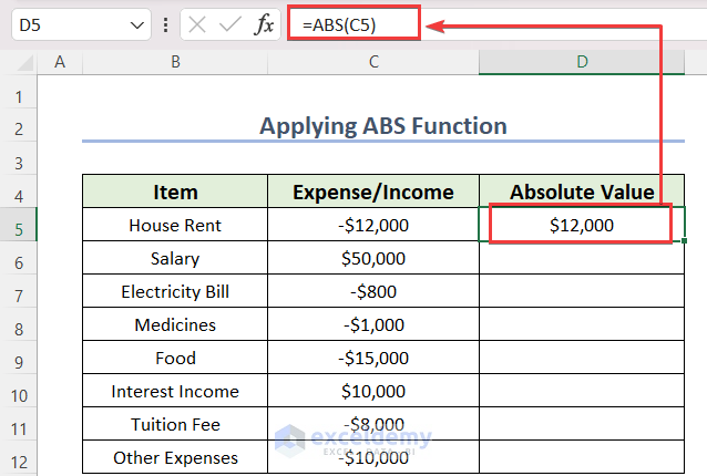
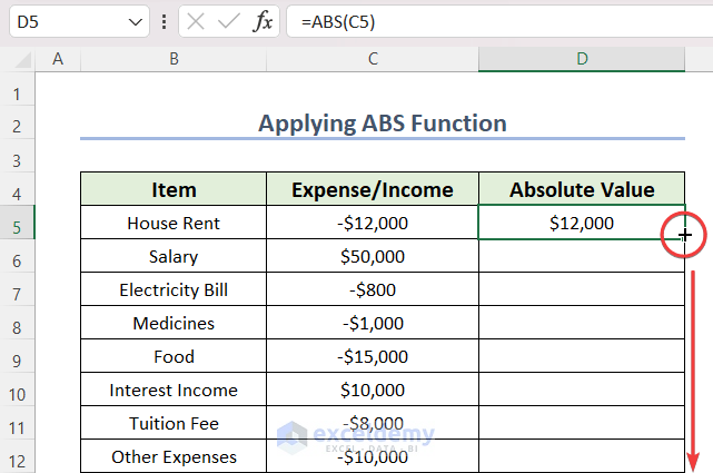
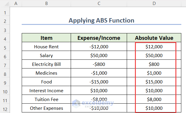
Example 5 – Using the ABS Function If a Cell Contains a Negative Number
Steps:
- Select a cell to see the result, here D5.
- Use the following formula in D5.
=ABS(C5)The ABS function returns the positive value of C5.
- Press ENTER.
- Drag down the Fill Handle to AutoFill the rest of the cells.
This is the output.
Read More: How to Add Negative Numbers in Excel
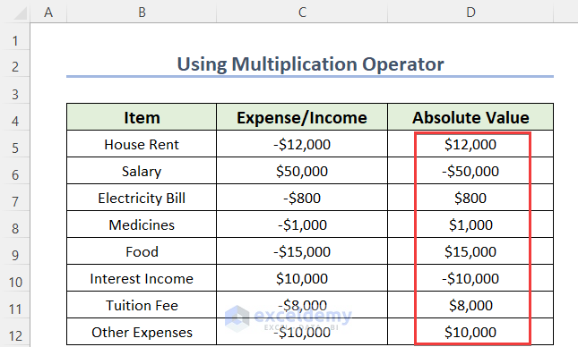
Example 6 – Applying the Multiplication (*) Operator in an Excel Formula
Steps:
- Select a cell to see the result, here D5.
- Use the following formula in D5.
=C5*-1The value C5 is multiplied by -1.
- Press ENTER.
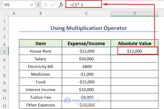
- Drag down the Fill Handle to AutoFill the rest of the cells.
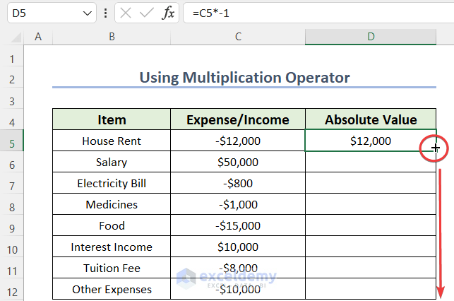
The positive numbers in column C become negative.
- Remove those numbers.
- Select the cells with negative values by pressing CTRL. Here, D6 and D10.
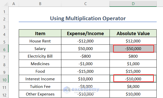
- Press DELETE.
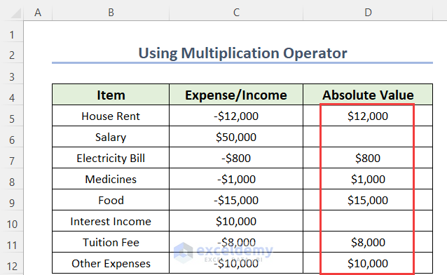
This is the output.
Read More: How to Make a Group of Cells Negative in Excel
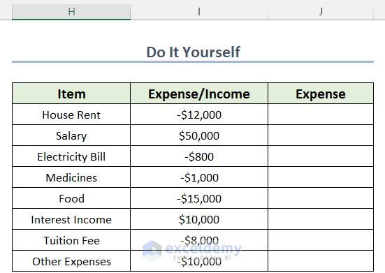
Practice Section
Practice here.
Download Practice Workbook
Download the practice workbook here:
Related Articles
<< Go Back to Negative Numbers in Excel | Number Format | Learn Excel
Get FREE Advanced Excel Exercises with Solutions!
