How to Make a Group of Cells Negative in Excel (5 Methods)

Here’s an overview of making the entire range get negative values.

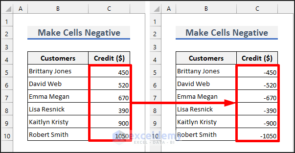
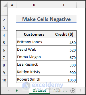
We will use a simple dataset with numeric values in column C.

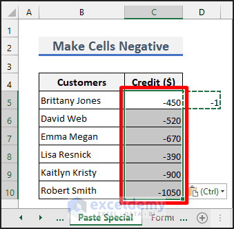
Method 1 – Using the Paste Special Tool to Make a Group of Cells Negative in Excel

Steps

• Enter -1 in an empty cell.
• Copy the cell.
• Select the group of cells that you want to make negative as shown in the following picture.

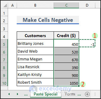
• Press Ctrl + Alt + V to open the Paste Special dialog box.
• Choose All except borders for Paste and Multiply for Operation.
• Hit the OK button.

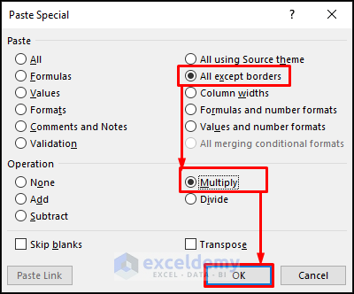
• Clear the cell containing -1.

Read More: How to Add Negative Numbers in Excel

Method 2 – Applying Excel Formula to Make a Group of Cells Negative

• Enter the following formula in cell D5.

• Apply the formula with Ctrl + Shift + Enter, or just Enter if you’re using Excel 365.

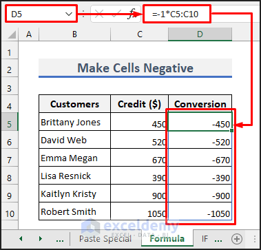
• You can copy the converted values and paste them as values on the Credit column and then delete the Conversion column.

Read More: [Fixed!] Excel Not Adding Negative Numbers Correctly

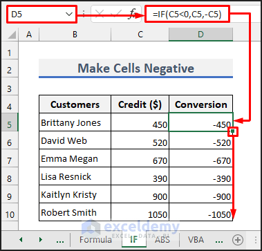
Method 3 – Inserting the IF Function to Convert a Group of Cells Negative

• Enter the following formula in cell D5.

• Apply it to the cells below using the fill handle tool.
• You can copy and paste as values to replace the original values.

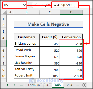
Method 4 – Making a Group of Cells Negative with the ABS Function

• Enter the following formula in cell D5.

• Apply the formula with Ctrl + Shift + Enter, or just Enter if you’re using Excel 365.

Read More: How to Put a Negative Number in Excel Formula

Method 5 – Using Excel VBA to Make a Group of Cells Negative

Steps

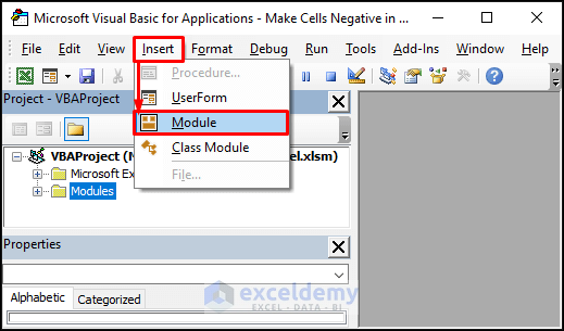
• Press Alt + F11 to open the Microsoft Visual Basic for Applications window.
• Select Insert and choose Module to open a new blank module.

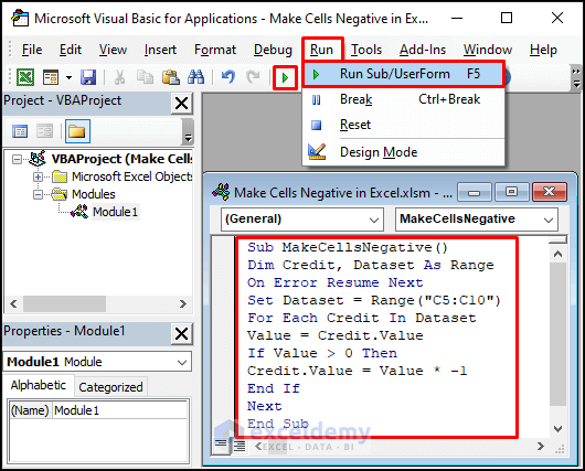
• Copy the following code.

Sub MakeCellsNegative()
Dim Credit, Dataset As Range
On Error Resume Next
Set Dataset = Range("C5:C10")
For Each Credit In Dataset
Value = Credit.Value
If Value > 0 Then
Credit.Value = Value * -1
End If
Next
End Sub

• Paste the copied code on the blank module.
• Press F5 to run the code.

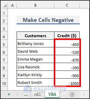
• The cells will show negative values as follows.

• You can repeatedly run the following code instead to make the cells negative or positive. Change the range in the code as needed.

Sub MakeCellsNegativeOrPositive()
Dim Credit, Dataset As Range
Set Dataset = Range("C5:C10")
For Each Credit In Dataset
Value = Credit.Value
Credit.Value = Value * -1
Next
End Sub

Read More: How to Show Negative Numbers in Excel

Download the Practice Workbook

Related Articles

• How to Count Negative Numbers in Excel
• Excel Formula to Return Zero If Negative Value is Found
• Excel Formula If Cell Contains Negative Number
• Excel Formula to Return Blank If Cell Value Is Negative

<< Go Back to Negative Numbers in Excel | Number Format | Learn Excel