How to Put a Negative Number in Excel Formula (4 Easy Methods)

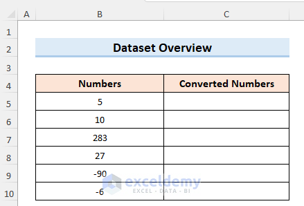
We’ll use a sample dataset with random numbers in one column and will then convert them to negative numbers in the other one by applying negative numbers in formulas.

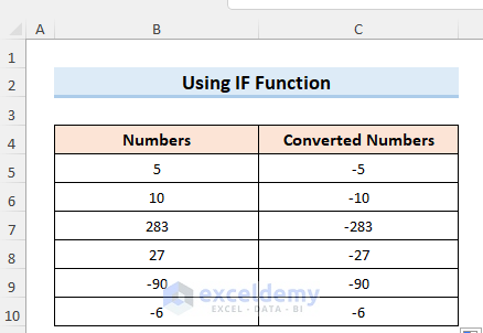
Method 1 – Applying the IF Function

Steps:

• Select C5.
• Insert the following formula in the selected cell.

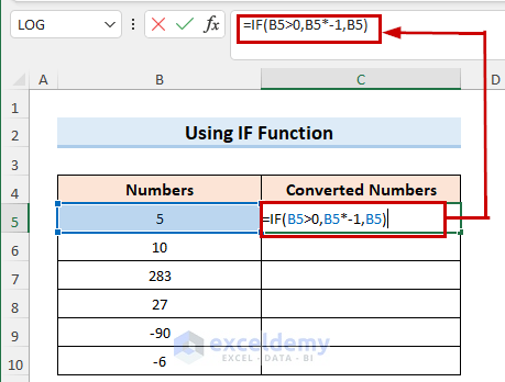
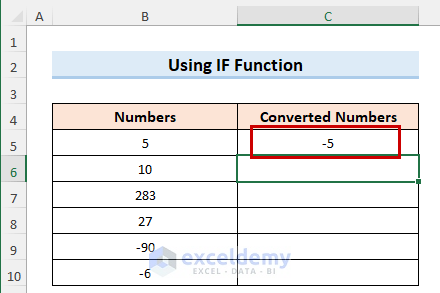
• Press the Enter button to get the result.

• Use the Fill Handle option to apply the formula to all cells in the column.

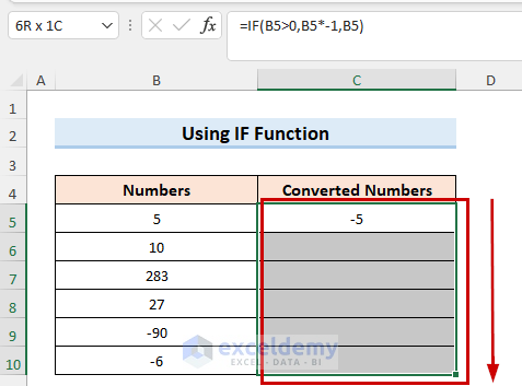
• You will get the final result similar to the below image.

Read More: How to Add Negative Numbers in Excel

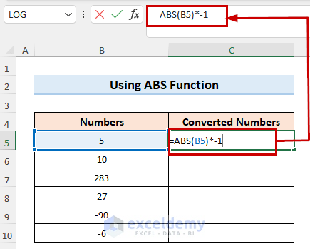
Method 2 – Use the ABS Function

Steps:

• Select C5 and insert the following formula
  
  =ABS(B5)*-1
  

• Use the Fill Handle to apply this formula to all the cells.

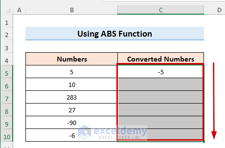
• Here are the results.

Read More: How to Show Negative Numbers in Excel

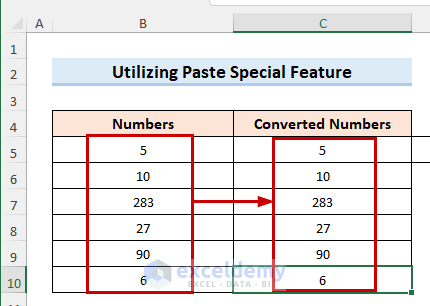
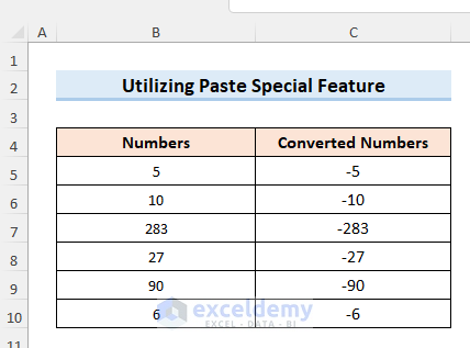
Method 3 – Utilizing Excel’s Paste Special Feature

Steps:

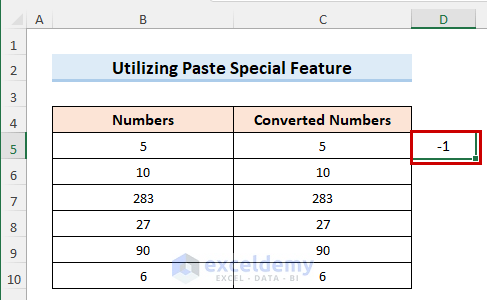
• Paste the numbers you want to convert into the desired column.

• Insert -1 into any blank cell (in this case cell D5) and copy the cell.

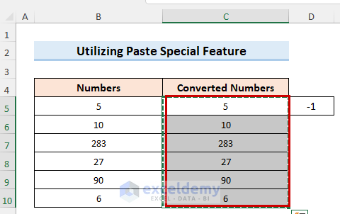
• Select the numbers you want to convert.

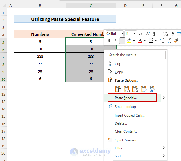
• Right-click on the column and choose the option Paste Special.

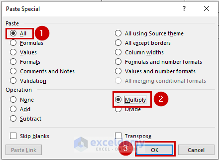
• The Paste Special dialog box will open.
• Select All in the Paste section and the Multiply option in the Operation section.
• Press OK.

• You will get the desired result.

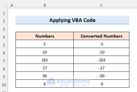
Method 4 – Applying VBA Code

Steps:

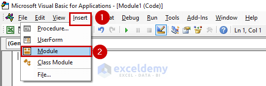
• Press Alt + F11 to open the VBA window.
• Go to Insert and select the Module option.

• Insert the following VBA code.

Sub Put_Negative_Number()
Dim wsheet As Worksheet
Dim rnge As Range
Dim rslt As Range
Set wsheet = Application.ActiveSheet
Set rnge = Application.Selection
For Each cell In rnge
If cell.Value > 0 Then
cell.Value = cell.Value * -1
End If
Next
End Sub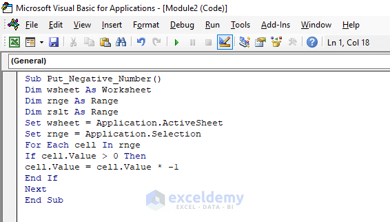

• Save the file as an .xlsm and go back to the sheet.
• Go to the Developer tab and use the Macros option to open the Macro tab.
• Select the macro and a range from the worksheet and press the Run option.

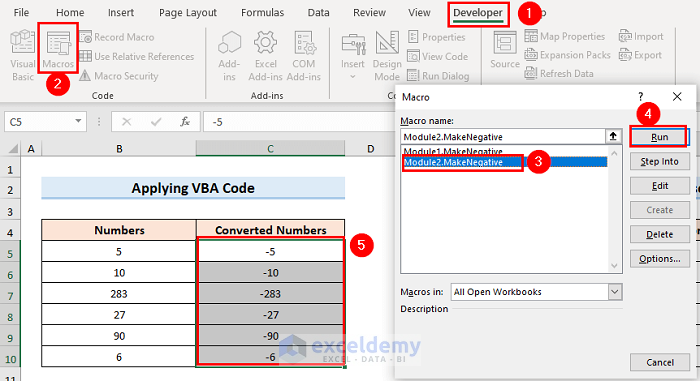
• Here are the results.

Read More: How to Make a Group of Cells Negative in Excel

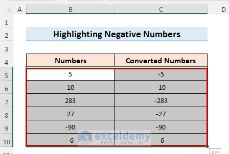
Highlighting Negative Numbers

Steps:

• Select the range of cells where you want to highlight negative numbers.

• Go to the Home tab and choose the Conditional Formatting option.
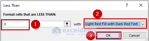
• Select the Less Than… option from the Highlight Cells Rules drop-down.

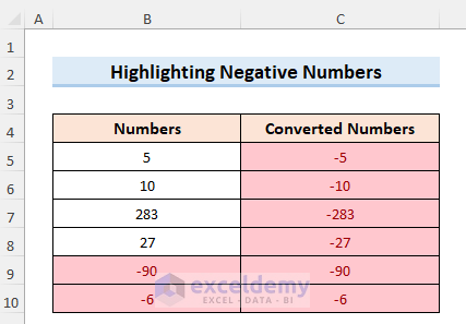
• Put 0 in Format cells that are Less THAN, select the desired formatting from the drop-down, and press OK.

• Here is the sample result.

Download the Practice Workbook

Related Articles

• How to Count Negative Numbers in Excel
• Excel Formula to Return Zero If Negative Value is Found
• Excel Formula If Cell Contains Negative Number
• Excel Formula to Return Blank If Cell Value Is Negative

<< Go Back to Negative Numbers in Excel | Number Format | Learn Excel