How to Add Negative Numbers in Excel – 4 Methods

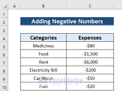
The sample dataset contains Categories and Expenses.

Method 1 – Using the SUMIF Function to Add Negative Numbers in Excel

Steps:

• Select a cell to see the result. Here, C11.
• Enter the formula in C11.

• Press ENTER to see the result.

This is the output.

Read More: How to Show Negative Numbers in Excel

Method 2 – Applying the AutoSum Feature to Add Negative Numbers

Steps:

• Select a cell to see the result. Here, C11.
• In the Home tab >> select Editing.
• In AutoSum >> choose SUM.

• Select the data range. Excel auto-selects the data range.

The Negative Number will be added.

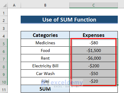
Method 3 – Use the Format Cells Command and the SUM Function to Add Negative Numbers in Excel

Steps:

•  Select the data range. Here, C5:C10.

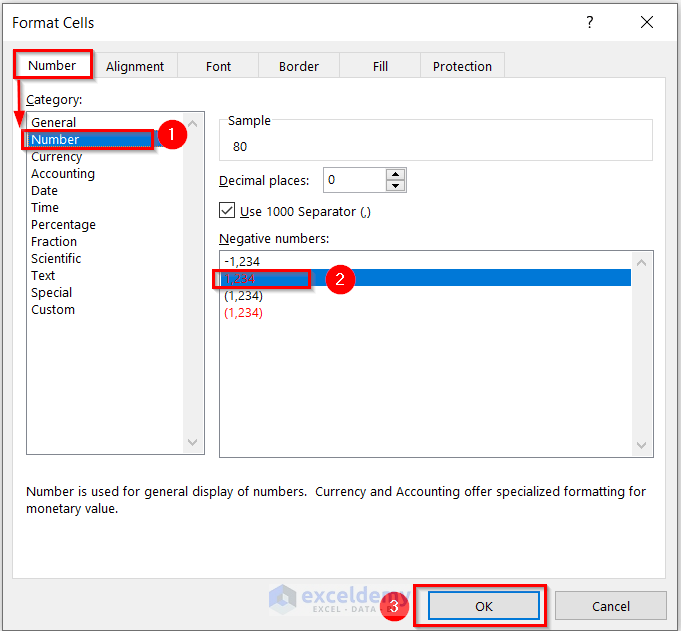
• Press  CTRL+1 to open the Format Cells dialog box.

You can use the Context Menu to go to the Format Cells command: select the data range >> Right-Click the data >> choose Format Cells.

You can use the Custom Ribbon:  select the data range >>in the Home tab >> go to Format >> choose Format Cells.

• In the dialog box, select Number.
• Choose Currency. Here, the dollar sign will be used for monetary values.
• In Negative numbers:  >> choose a style. Here, the 2nd style.
• Click OK to see the changes.

To keep the data as numbers only, use the Number format.

• Go to Number.
• In Negative numbers: >> choose a style.
• Click OK.

This will be the output.

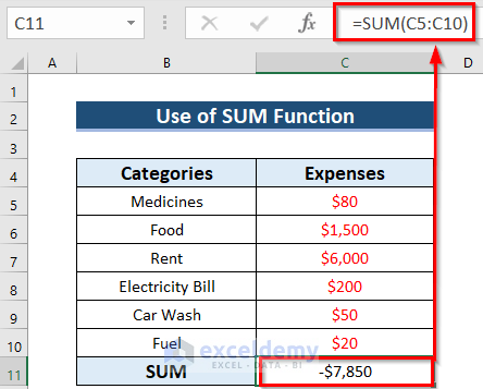
• Select a different cell: C11, to keep the result.
• Enter the formula in C11.

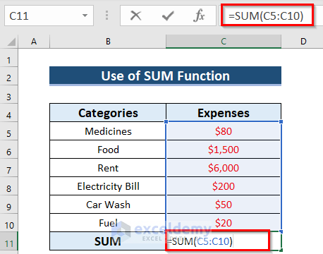
The SUM function will sum all the numbers in C5:C10.

• Press ENTER.

This is the output.

Read More: How to Put a Negative Number in Excel Formula

Method 4 – Using a Generic Formula to Add Negative Numbers in Excel

Steps:

• Select a cell to see the result. Here, C11.
• Enter the formula in C11.

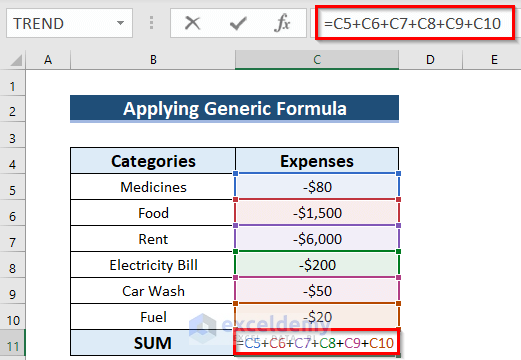
The Plus (+) sign was added to cell values.

• Press ENTER.

This is the output.

Read More: How to Make a Group of Cells Negative in Excel

Things to Remember

• When there are both positive and negative numbers and you want to add negative numbers only, use the SUMIF function (method 1).
• When you have only negative numbers, use either method 2 or method 3.

Download Practice Workbook

Download the practice workbook.

Related Articles

• How to Count Negative Numbers in Excel
• Excel Formula to Return Zero If Negative Value is Found
• Excel Formula If Cell Contains Negative Number
• Excel Formula to Return Blank If Cell Value Is Negative

<< Go Back to Negative Numbers in Excel | Number Format | Learn Excel