This is an overview.
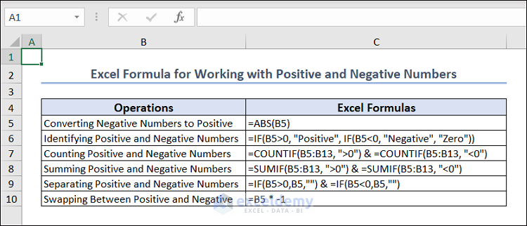
Overview of Excel Formulas for Working with Positive and Negative Numbers
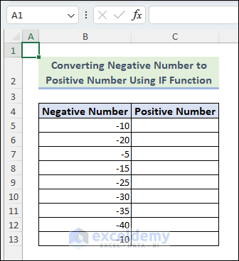
Example 1 – Converting Negative Numbers to Positive Numbers Using Excel Formulas
1.1 Using the Excel IF Function
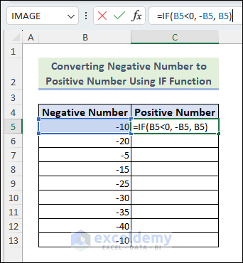
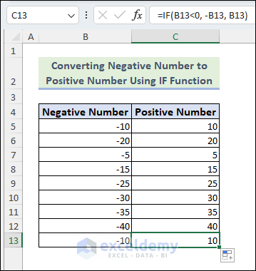
There are negative values in B5:B13 under the heading Negative Number. To convert these negative values and store them in column C (Positive Number):
Step 1:
- Select C5 => Enter the following formula:
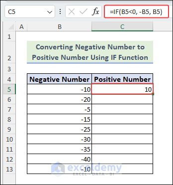
=IF(B5<0, -B5, B5)
Step 2:
- Press Enter or Tab.
-10 is converted to 10.
Step 3:
- Hover the cursor over the bottom right corner of C5 => You will see the Fill Handle icon.
![]()
Step 4:
- Drag the Fill Handle to convert the rest of the negative values to positive values.
You can also double-click the Fill Handle to copy the formula to the other cells in the column.
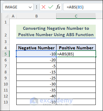
1.2 Using the Excel ABS Function
Step 1:
- Select C5 => Use the below formula:
=ABS(B5)
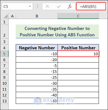
Step 2:
- Press Enter.
-10 is converted to 10.
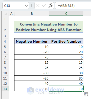
Step 3:
- Find the Fill Handle icon.
![]()
Step 4:
- Drag down the Fill Handle to see the result in the rest of the cells.
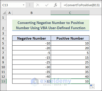
1.3 Using the Excel VBA User-Defined Function
Step 1:
- Go to the Developer tab => In Code, select Visual Basic.
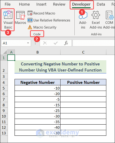
Step 2:
- Click Visual Basic to open the VBA Editor window => Select Insert => Click Module => Enter the following code in the module, and Save.
Function ConvertToPositive(ByVal num As Double) As Double

    If num < 0 Then
        ConvertToPositive = -num
    Else
        ConvertToPositive = num
    End If

End Function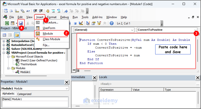
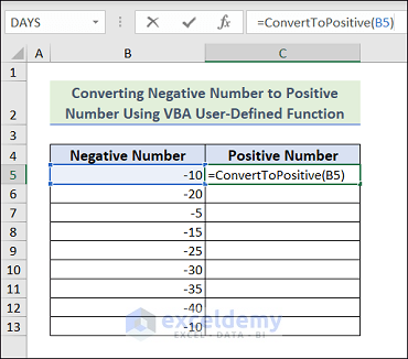
Step 3:
- Go back to to the sheet and select C5 => Enter the following:
=ConvertToPositive(B5)
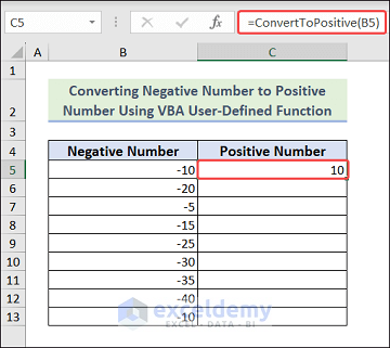
Step 4:
- Press Enter.
-10 is converted to 10.
Step 5:
- Find the Fill Handle.
![]()
Step 6:
- Double-click the Fill Handle to copy the formula to the other cells.
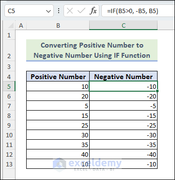
If you need to convert positive to negative numbers, use the Excel IF function.
Excel Formula to convert positive to negative values:
=IF(B5>0, -B5, B5)
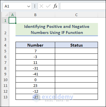
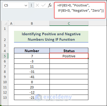
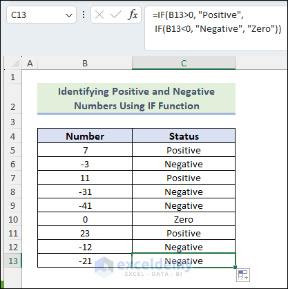
Example 2 – Identifying Positive and Negative Numbers Using the IF Function
To identify positive and negative numbers and place them in the Status column.
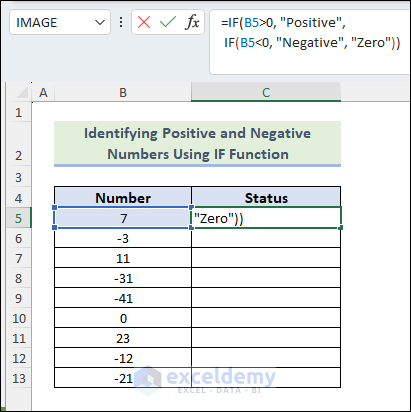
Step 1:
- Select C5 => use the following formula:
=IF(B5>0, "Positive", IF(B5<0, "Negative", "Zero"))
Step 2:
- Press Enter.
7 is displayed as a positive number.
Step 3:
- Find the Fill Handle icon.
![]()
Step 4:
- Drag down the Fill Handle to see the result in the rest of the cells.
Read More: How to Make Negative Numbers Red in Excel
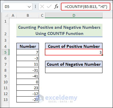
Example 3 – Counting Positive and Negative Numbers Using the COUNTIF Function
To count and store the value of positive numbers in D6 and negative numbers in D8:
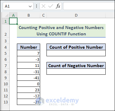
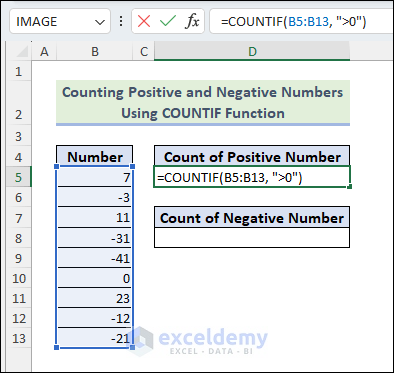
To count the positive numbers:
Step 1:
- Select D5 => Enter the following formula:
=COUNTIF(B5:B13, ">0")
Step 2:
- Press Enter.
3 is displayed in D5, as there are only three positive numbers.
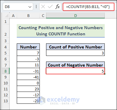
To count the negative numbers:
Step 3:
- Select D8 =>Enter the following formula:
=COUNTIF(B5:B13, "<0")
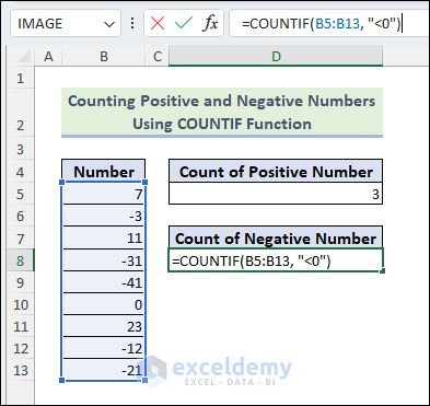
Step 4:
- Press Enter.
5 is displayed in D8, as there are five negative numbers.
Read More: How to Sum Negative and Positive Numbers in Excel
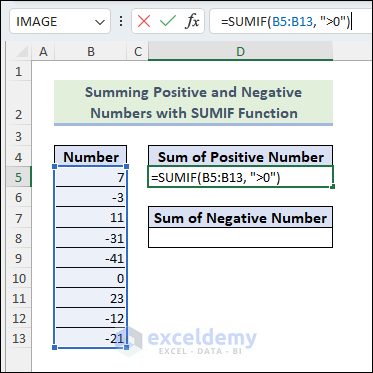
Example 4 – Summing Positive and Negative Numbers with the SUMIF Function
To store the summation of positive and negative numbers in D5 and D8.
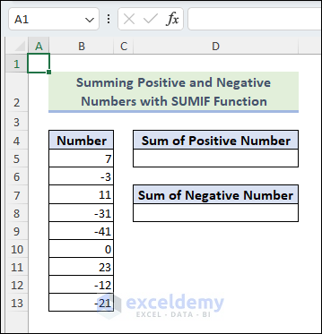
Sum the positive numbers.
Step 1:
- Select D5 =>Use the following formula:
=SUMIF(B5:B13, ">0")
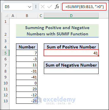
Step 2:
- Press Enter.
41 is displayed in D5.
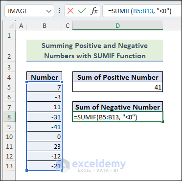
Sum the negative numbers.
Step 3:
- Select D8 =>Enter the following formula:
=SUMIF(B5:B13, "<0")
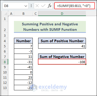
Step 4:
- Press Enter.
-108 is displayed in D8.
Read More: How to Put Negative Percentage Inside Brackets in Excel
Example 5 – Separating Positive and Negative Numbers Using Excel Formulas
5.1 Using MAX and MIN Functions
To keep all positive and negative numbers in columns D and E:
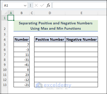
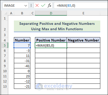
Separate all positive numbers.
Step 1:
- Choose D5 => Enter the following formula:
=MAX(B5,0)
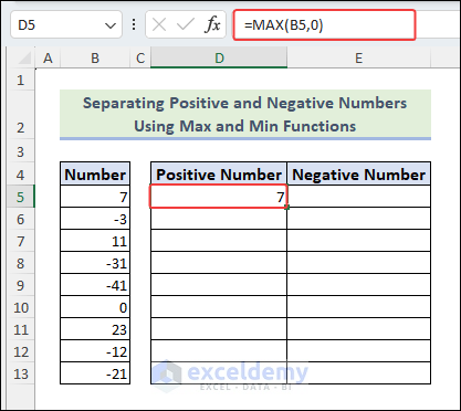
Step 2:
- Press Enter.
7 is displayed in D5.
Step 3:
- Find the Fill Handle.
![]()
Step 4:
- Drag down the Fill Handle to see the result in the rest of the cells.
![]()
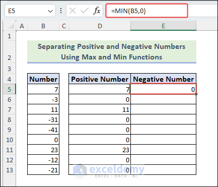
To separate the negative numbers.
Step 5:
- Select E5 => Use the following formula:
=MIN(B5,0)
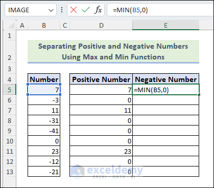
Step 6:
- Press Enter.
0 is displayed in E5.
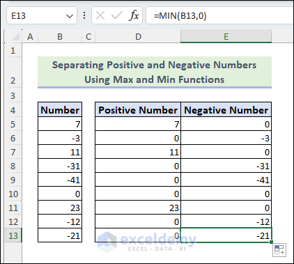
Step 7:
- Find the Fill Handle.
![]()
Step 8:
- Drag down the Fill Handle to see the result in the rest of the cells.
Separating positive and negative numbers with the MAX and the MIN functions inserts a 0 in the cells. To avoid it, use the IF function.
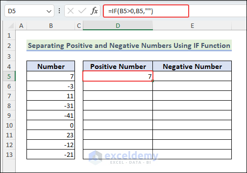
5.2 Using the IF Function
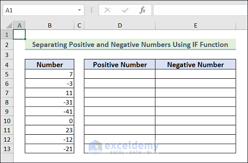
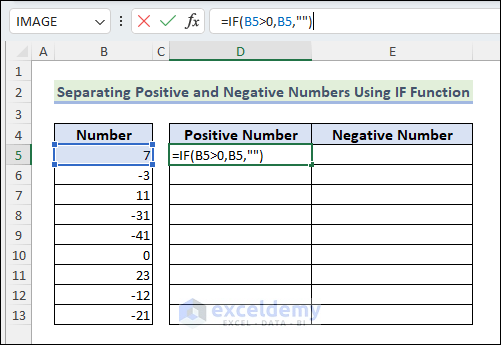
Separate positive numbers.
Step 1:
- Select D5 => Enter the following formula:
=IF(B5>0,B5,"")
Step 2:
- Press Enter.
7 is displayed in D5.
Step 3:
- Find the Fill Handle.
![]()
Step 4:
- Drag down the Fill Handle to see the result in the rest of the cells.
Positive numbers are separated and there are no extra zeros.
![]()
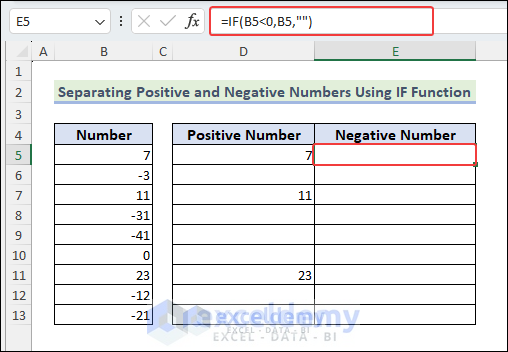
Separate the negative numbers.
Step 5:
- Select E5 => Enter the following formula:
=IF(B5<0,B5,"")
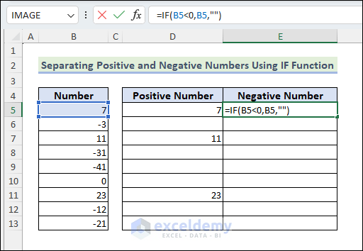
Step 6:
- Press Enter.
E5 is empty.
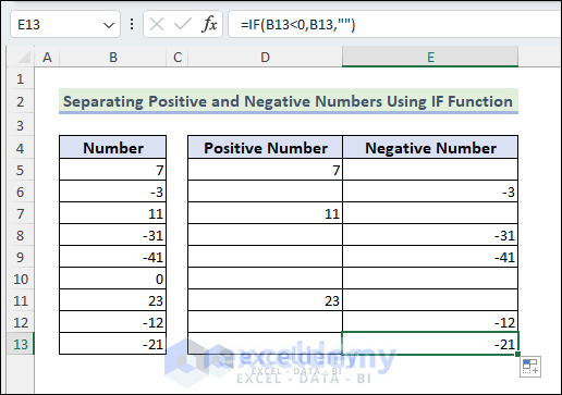
Step 7:
- Find the Fill Handle.
![]()
Step 8:
- Drag down the Fill Handle to see the result in the rest of the cells.
Negative numbers are separated and there are no extra zeros.
Read More: How to Add Brackets to Negative Numbers in Excel
Example 6 – Swapping Between Positive and Negative Numbers By Multiplying Negative – 1
To swap positive and negative numbers and place them in E5:E13:
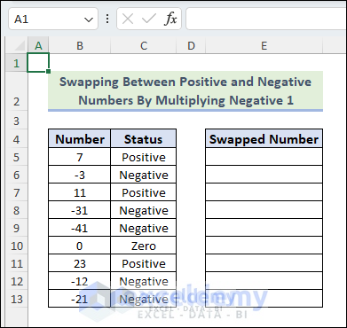
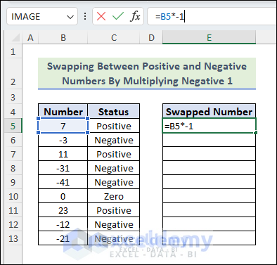
Step 1:
- Select E5 =>Enter the following formula:
=B5 * -1
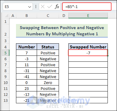
Step 2:
- Press Enter.
7 is turned into -7 in E5.
Step 3:
- Find the Fill Handle.
![]()
Step 3:
- Drag down the Fill Handle to see the result in the rest of the cells.
All numbers are swapped.
![]()
Read More: How to Move Negative Sign at End to Left of a Number in Excel
Download Practice Workbook
Related Articles
- Excel Negative Numbers in Brackets and Red
- How to Put Parentheses for Negative Numbers in Excel
- How to Change Positive Numbers to Negative in Excel
<< Go Back to Negative Numbers in Excel | Number Format | Learn Excel
Get FREE Advanced Excel Exercises with Solutions!
