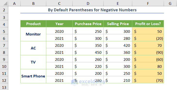
The following sample dataset of Purchase Price and Selling Price are provided in USD for each Product. If you subtract the Selling Price from the Purchase Price (=E5-D5 for the F5 cell), the value is Profit. A negative value will be found if there is a Loss.
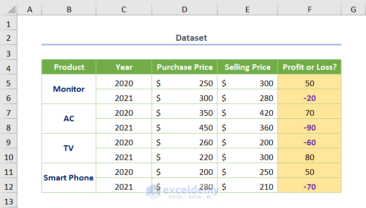
We will insert a parentheses for the negative values.
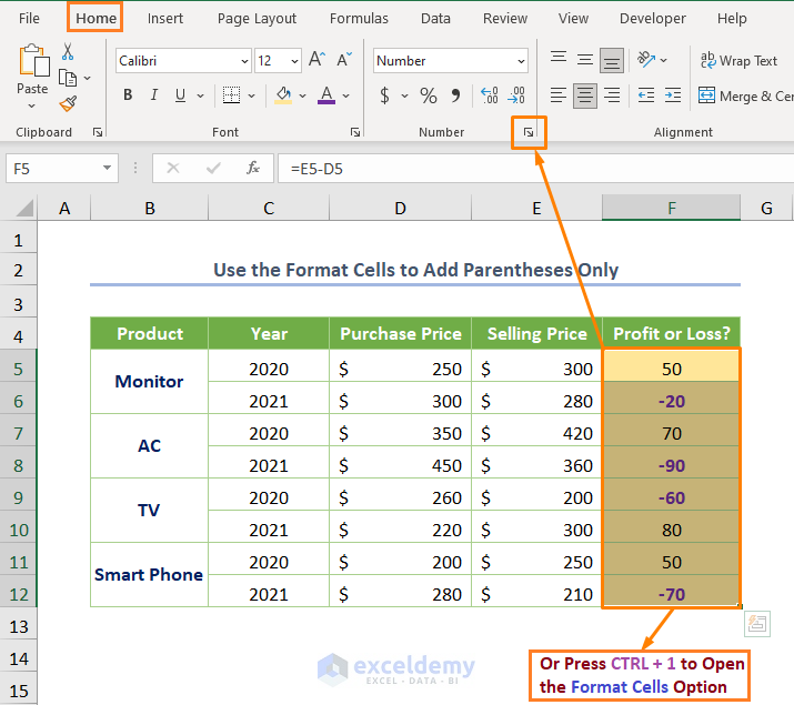
Method 1 – Using Excel Format Cells Dialog Box to Put Parentheses for Negative Numbers
- Select the number values, (F5:F12 cell range).s, Right-click, select Format Cells option from the Context Menu.
- You may click on the arrow of the Number Format option from the Home tab to go to the option directly.
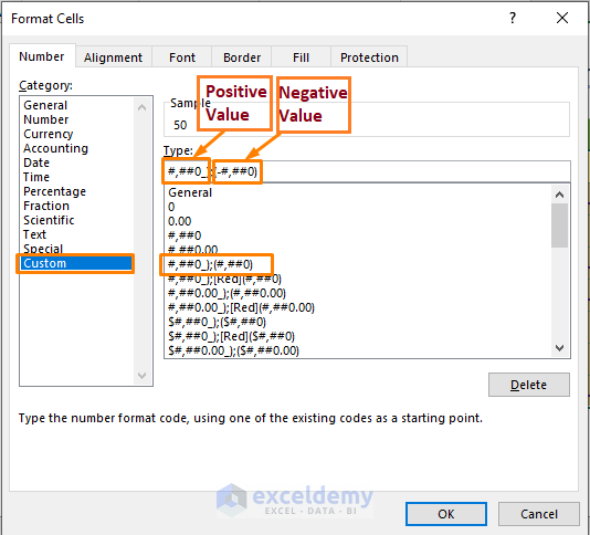
In the dialog box, select the number (1.234) format from the Negative numbers option under Number category.
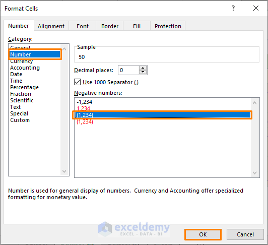
Click OK.
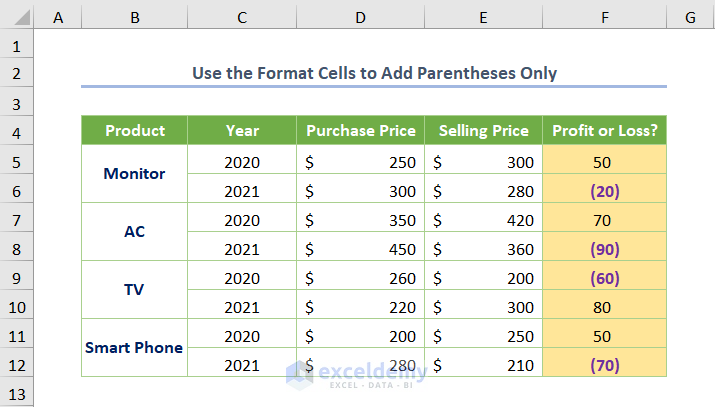
Note: If you’re a Microsoft 365 user, you’ll see the negative numbers with parenthesis by default as shown in the following image.
Read More: How to Custom Cell Format Number with Text in Excel (4 Ways)
Method 2 – Setting Parentheses with Negative Sign in Excel
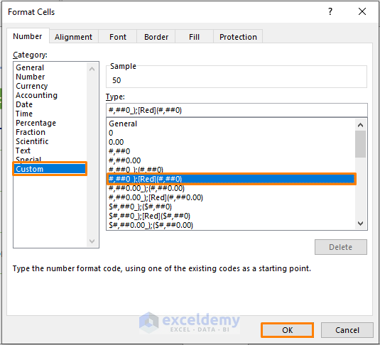
Select the cells, go to Format Cells.
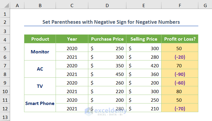
Select Custom option from the Category. Pick the format code #,##0_);(#.##0) and insert the minus sign as shown below. The format code will be:
#,##0_);(-#.##0)
The two format codes are combined. The first one refers to positive values whereas the second one is for negative values with parentheses. When you include the minus sign, the second format code will add the sign as well as keep the parentheses for your negative values.
You’ll get the following output.
Read More: Excel Custom Number Format Multiple Conditions
Similar Readings
- How to Format Number to Millions in Excel (6 Ways)
- [Fixed!] Excel Not Recognizing Numbers in Cells (3 Techniques)
- How to Change Comma to Dot in Excel (4 Handy Ways)
- How to Apply Number Format in Millions with Comma in Excel (5 Ways)
- Excel Number Stored As Text [4 Fixes]
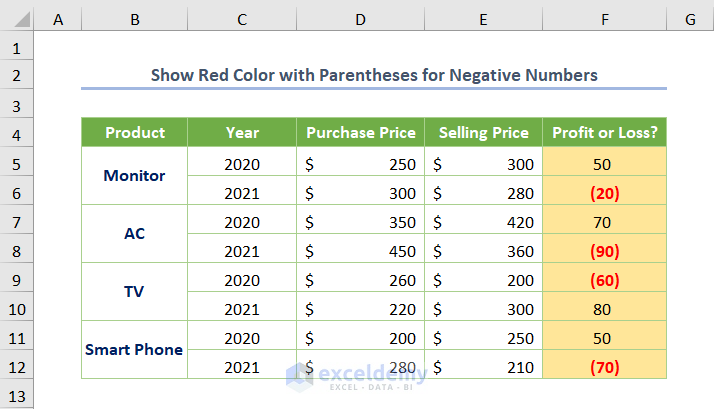
Method 3 – Showing Red Color in Excel with Parentheses for Negative Numbers
To highlight the negative number with the defined color, select the following format code from the Custom category.
#,##0_);[Red](#,##0)
The word [Red] displays the negative numbers in red font color.
The output will be as shown.
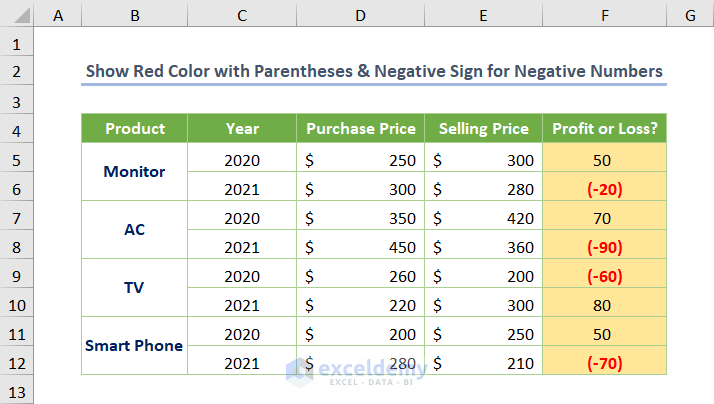
If you want to show a negative sign along with the red color and parentheses, you need to insert the sign after [Red] as depicted in the following image.
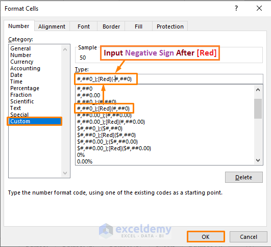
You’ll get your desired output.
Read More: How to Format Number with VBA in Excel (3 Methods)
How to Fix If Negative Numbers Don’t Show with Parentheses in Excel
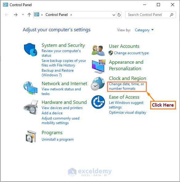
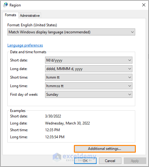
While placing the parentheses in Excel for negative numbers, you might get an error even if you tried all the methods. If you are a macOS user, update the OS. If you are a Windows OS user, go to the Control Panel and click on the Change date, time or number formats under the Clock and Region settings.
Click on Additional settings from the Formats tab.
Click on the drop-down list (located on the right side of the Negative number format option). Select (1.1) as the format.
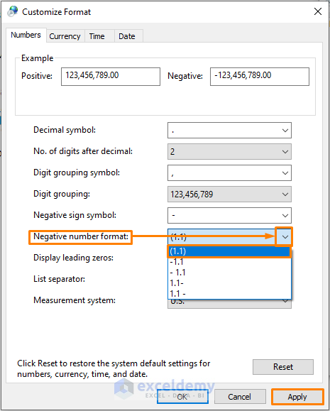
Click Apply.
Download Practice Workbook
Related Articles
- Excel Round to Nearest 100 (6 Quickest Ways)
- Excel 2 Decimal Places without Rounding (4 Efficient Ways)
- How to Use Phone Number Format in Excel (8 Examples)
- How to Custom Format Cells in Excel?
- Keep 0 Before a Phone Number in Excel (6 Methods)


This procedure for displaying negative numbers in parentheses did not work for me. I can use the ‘Format cell’ routine for individual spreadsheets with no problem but I could not get the ‘Control Panel’ procedure to change the environment globally: each new spreadsheet reverts to displaying the minus sign.
I’m using Excel 2013 under Windows 10 which I keep routinely updated.
Dear William Moloney,
As far as I understand, you are able to use “Format Cell” but can’t get the procedure of using “Control Panel” to fix negative number format, right?
You are using Windows 10 and you can do it easily in Windows 10.
Firstly, go to “Control Panel”.
Secondly, click on “Change date, time and number format” in the option “Clock and Region”.
Thirdly, a window named “Region” will appear. Go to “Formats” option of that window. Click on “Additional settings” at the right-bottom side of the window.
You will see a “Customize Format” window. Go to “Numbers” of this window. You’ll see many options available in this “Numbers” option.
Fourthly, in the “Negative Number Format” option, click on the value and you will see different options such as 1.1, -1.1, 1.1- etc. You need to select 1.1 here and then click OK. This is the most important step here to select 1.1. Windows 10 has default selection 0f -1.1, you need to just change it to 1.1.
Hope, your problem will be solved now. Thank you.
Regards,
Towhid
Excel & VBA Content Expert
ExcelDemy