The following GIF shows that the custom number format is changing based on multiple conditions. Depending on the values you enter in the cell, the Delta or Inverted Delta symbols will be added at the end.
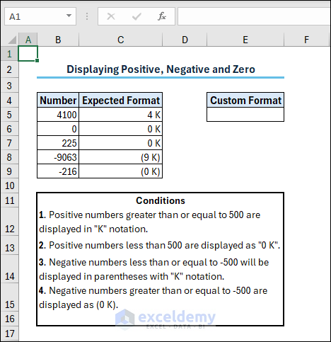
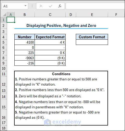
Displaying Positive, Negative, and Zero
The dataset’s right-side column shows an Expected Format for a series of numbers. This formatting will follow some conditions:
- Positive numbers ≥ 500 appear as “K”.
- Positive numbers < 500 show as “0 K”.
- Negative numbers ≤ -500 are displayed in “(K)” format.
- Negative numbers > -500 are shown as “(0 K)”.
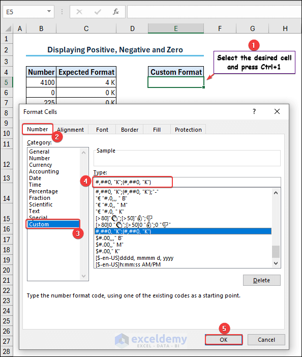
Steps:
- Select your desired cell.
- Press Ctrl+1 to open the Format Cells dialog box.
- In the Format Cells dialog box:
- Go to the Number tab.
- Click on Custom from the Category section.
- Enter the following format code in the Type field:
#,##0, "K";(#,##0, "K") - Press OK.
As a result, you will see an output applying a custom number format with multiple conditions like the following GIF.
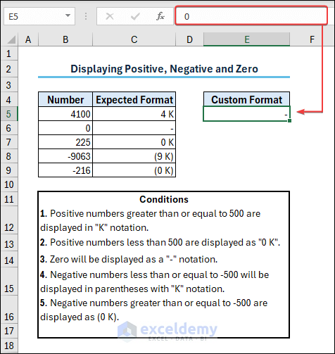
Displaying a Dash as Zero
- Enter the formatting code:
#,##0, "K";(#,##0, "K");"-"
You will see the intended output as follows:
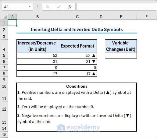
Inserting a Delta and Inverted Delta Symbols
Assume you want a custom number format for increasing or decreasing units with Delta and Inverted Delta symbols like the following screenshot. The idea here will maintain the following conditions:
- Positive numbers are marked with a Delta (▲) symbol.
- Zero is presented as the number 0.
- Negative numbers feature an Inverted Delta (▼) symbol.
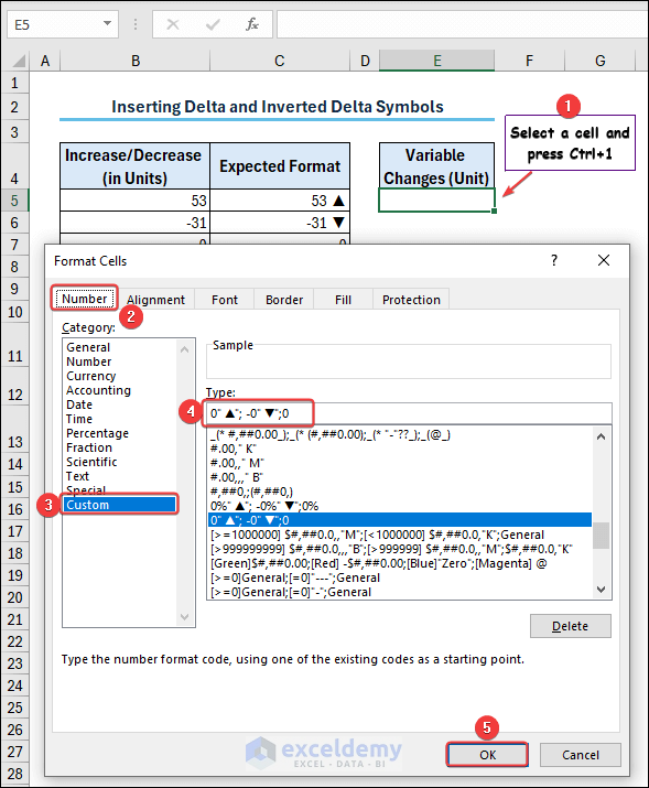
Steps:
- Select an empty cell.
- Press Ctrl+1 to open the Format Cells dialog box.
- In the Format Cells dialog box:
- Go to the Number tab.
- Click on Custom from the Category section.
- Enter the following format code in the Type field:
0" ▲"; -0" ▼";0 - Press OK.
As a result, you will see an output displaying delta and inverted delta based on conditions like the following GIF.
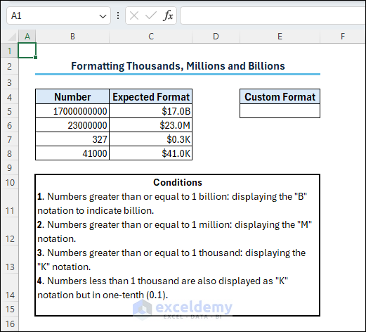
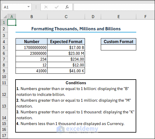
Formatting Thousands, Millions and Billions
When working with large numbers, you can display numbers in billion, million, and thousand formations. The idea can be done using a custom number format like the following image. However, you must apply several conditions to the formatting code. Here are the conditions:
- ≥ 1 billion: “B” notation.
- ≥ 1 million: “M” notation.
- ≥ 1 thousand: “K” notation.
- < 1 thousand: “K” notation with one-tenth (0.1) formation.
Steps:
- Select an empty cell.
- Press Ctrl+1 to open the Format Cells dialog box.
- In the Format Cells dialog box:
- Go to the Number tab.
- Click on Custom from Category.
- Enter the following format code in the Type field:
[>999999999] $#,##0.0,,,"B";[>999999] $#,##0.0,,"M";$#,##0.0,"K" - Press OK.
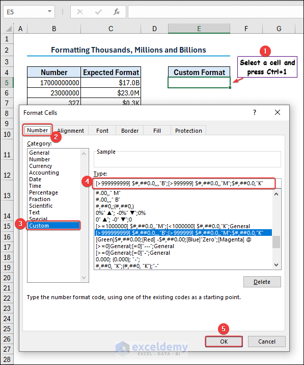
- Insert multiple large numbers and see an output like the GIF below.
Displaying Numbers Less Than 1000 as General Format
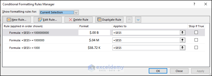
Assume you are in a situation where you do not want to display the “K” notation for values less than one thousand, like the screenshot below.
Unfortunately, only using a custom number format to perform such a task is very difficult. However, you can apply multiple conditional formattings in a cell so that if the values are less than one thousand, it will be formatted like regular currency.
Steps:
- Apply the currency format in an empty cell.
- Apply the following three conditional formatting and three format codes in the cell:
- Formula 1:
=$E$5>=1000000000 - Format Code 1:
$#.00,,," B" - Formula 2:
=$E$5>=1000000 - Format Code 2:
$#.00,,"M" - Formula 3:
=$E$5>=1000 - Format Code 3:
$#.00,,"K"
- Formula 1:
It is important to remember that you must prioritize the conditional formatting rules from the highest to the lower order, which means the formula for billions will be at the top, later comes the millions formula, and lastly, for thousands.
You will see an output like the GIF below.
Read More: How to Format a Number in Thousands K and Millions M in Excel
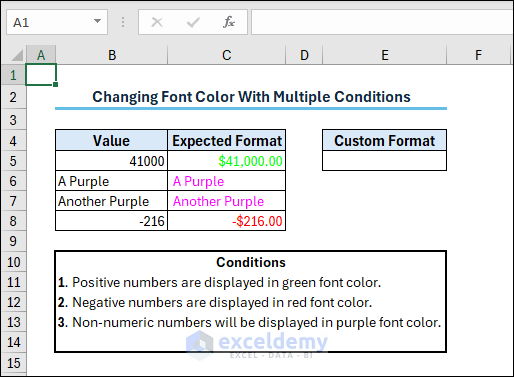
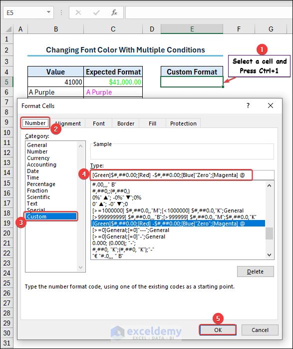
Changing Font Color With Multiple Conditions
You can customize a number format code to change the font color based on several conditions. Assume you want to use green font for positive numbers and red font for negative numbers. If the cell value is text, the font color will be purple, as in the following screenshot.
Steps:
- Select your desired cell.
- Press Ctrl+1 to open the Format Cells dialog box.
- In the Format Cells dialog box:
- Go to the Number tab.
- Click on Custom from the Category.
- Enter the following format code in the Type field:
[Green]$#,##0.00;[Red] -$#,##0.00;[Blue]"Zero";[Magenta] @ - Press OK.
You will get an output like the following GIF.
Read More: How to Apply Number Format in Millions with Comma in Excel
Displaying an Emoji With Multiple Conditions
You can insert various emojis in a custom number format based on multiple conditions. Assume you have a dataset like the following image where you want to format student marks, including some thumb emojis at the end.
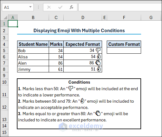
In this case, you have to create a custom format keeping the following conditions in mind:
- Marks less than 50: An “” emoji will be included at the end to indicate a lower performance.
- Marks between 50 and 79: An “” emoji will be included to indicate an acceptable performance.
- Marks equal to or greater than 80: An “” emoji will be included to indicate an excellent performance.
Note: To insert an emoji in Windows OS, press the Windows+. or Windows+; keys. It is important to note that these emojis will be displayed as greyscale on the Excel Desktop. However, you will find the emojis with their colored glory in Excel Online.
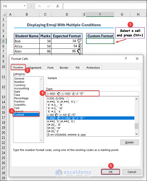
Steps:
- Select an empty cell.
- Press Ctrl+1 to open the Format Cells dialog box.
- In the Format Cells dialog box:
- Go to the Number tab.
- Click on Custom from the Category section.
- Enter the following format code in the Type field:
[>80]0 "";[>50]0 "";0 ""
You can modify the formatting code for other conditions. For example, insert the desired condition within the square bracket [> 60]. - Press OK.
You will see the intended emoji will be displayed and get an output like the following GIF.
Read More: How to Add Number with Text in Excel Cell with Custom Format
Download the Practice Workbook
Related Articles
- Excel Custom Number Format – Millions with One Decimal
- How to Apply Custom Format Cells in Excel
- How to Format Number to Millions in Excel
- How to Add Text after Number with Custom Format in Excel
<< Go Back to Custom Number Format | Number Format | Learn Excel
Get FREE Advanced Excel Exercises with Solutions!

Good.
Thanks for your feedback.
Interesting but I have not used it before.
Thanks for early training articles to equip one at the right time.
Thanks once again
Thanks for the feedback. Hope you will find this technique useful for your next some jobs.
Best regards
Kawser Ahmed
Thanks a lot sir for simple explanation and illustrations.