To apply a custom format in Excel:
- Select the cell or range you want to format.
- Press Ctrl + 1 to open the Format Cells dialog box.
- In the Format Cells dialog box:
- Click Custom from the Category.
- In the Type field, select the format that you created.
- Hit OK.
How Does a Custom Format Work in Excel Cells?
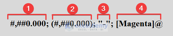
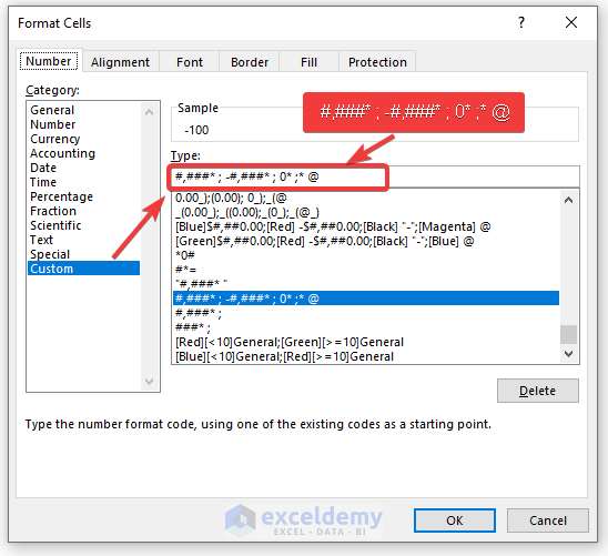
A custom format consists of 4 sections of code. In the following image, you can see that semicolons separate these codes.

Here’s a breakdown of each option:
- For Positive numbers (display 3 decimal places and a thousand separator).
- In the case of the negative numbers (enclosed in parenthesis).
- For zeros (display dashes instead of zeros).
- Text values format.
Formatting Guidelines and Considerations
You can create multiple custom number formats in Excel by applying the formatting codes mentioned in the table below. The following hints will show you how to utilize these format codes in the most usual and practical ways.
| Format Code | Description |
|---|---|
| General | number format |
| # | Digit placeholder which does not show extra zeros and symbolizes optional digits. |
| 0 | Unimportant zeros are represented in a digit placeholder. |
| ? | A digit placeholder, which leaves a place for them but does not show them, hides unimportant zeros. |
| @ | Text placeholder |
| (. )(Dot) | Decimal point |
| (,) (Comma) | Separator for thousands. After a digit placeholder, a comma represents the numbers multiplied by a thousand. |
| \ | The character that comes after it is shown. |
| ” “ | Any text wrapped in double quotes will be shown. |
| % | The percentage indication is presented after multiplying the values input in a cell by 100. |
| / | Specifies fractions as decimal numbers. |
| E | Specifies the format for indicating scientific notation. |
| (_ ) (Underscore) | Bypasses the following character’s width. |
| (*) (Asterisk) | Continue with the next character until the cell is entirely filled. It’s typically paired with another space character to adjust alignment. |
| [ ] | It is used to make use of conditional formatting. |
Characters that Display by Default
Some characters appear in numerical format by default, while others require specific treatment. The following characters can be used without any special handling.
| Character | Description |
|---|---|
| $ | Dollar |
| +- | Plus, minus |
| () | Parentheses |
| {} | Curly braces |
| <> | Less than, greater than |
| = | Equal |
| : | Colon |
| ^ | Caret |
| ‘ | Apostrophe |
| / | Forward slash |
| ! | Exclamation point |
| & | Ampersand |
| ~ | Tilde |
| Space character |
How to Custom Format Cells in Excel: 17 Examples
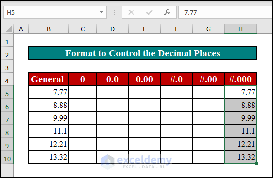
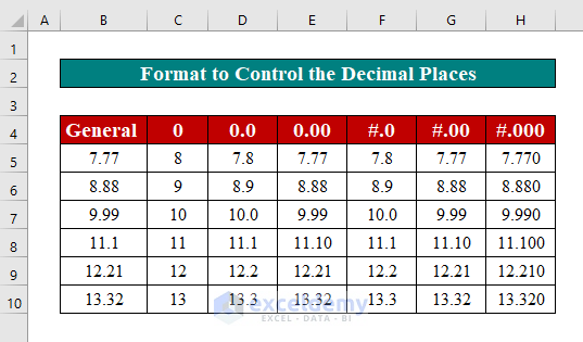
Example 1 – Controlling Decimal Places in Numbers
A period (.) represents the decimal point’s location. The number of decimal places required is determined by zeros (0). Some format examples: 0 or # – shows the nearest integer with no decimal places; 0 or #.0 – shows 1 decimal place; 00 or #.00 – shows 2 decimal places.
- Select the cells for which you want to create custom formatting.
- Press Ctrl + 1 to open the Format Cells dialog box.
- In the Format Cells dialog box:
- Under Category, select Custom.
- Write the format code in the Type field:
#.000 - Hit OK.
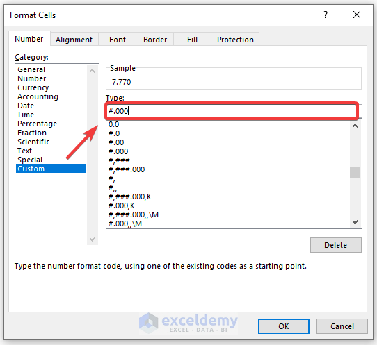
- The selected cell will be formatted with three decimal places.
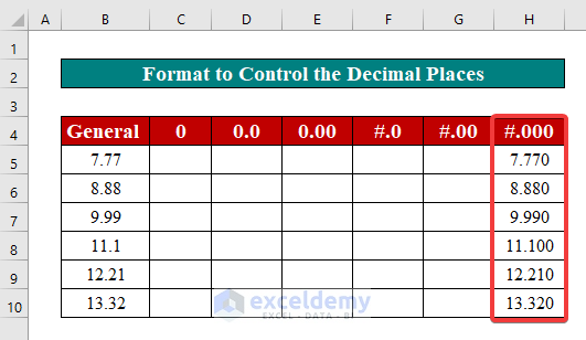
- Repeat the steps and type different format codes individually to display other decimal places.
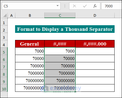
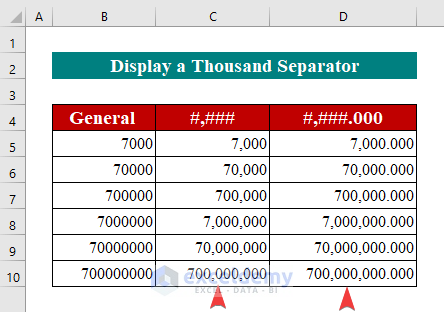
Example 2 – Showing the Thousand Separator in Excel Cells
You can use a comma (,) in the format code to generate a custom number format with a thousand separator. Some format examples include #,### – display a thousand separators and no decimal places; #,##0.000 – display a thousand separators and 3 decimal places.
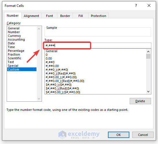
- Select cells for which you want to create custom formatting.
- Press Ctrl + 1 to open the Format Cells dialog box.
- In the Format Cells dialog box:
- From the Category section, select Custom.
- Write the format code in the Type field:
#,### - Press OK.
- You will see that cells are formatted like the following image.
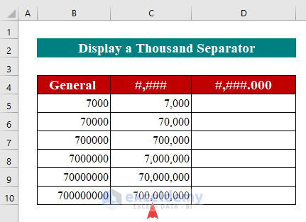
- Repeat the steps and use the corresponding format code to display the other format.
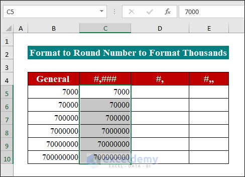
Example 3 – Rounding Numbers with a Custom Format
You can use commas with any numeric placeholders like pound symbol (#), question mark (?), or zero (0) in a format code when rounding large numbers.
- Select cells for which you want to create custom formatting.
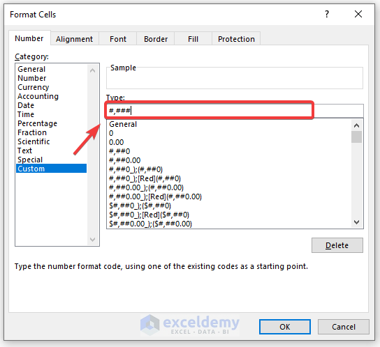
- Press Ctrl + 1 to open the Format Cells dialog box.
- In the Format Cells dialog box:
- Select Custom from the Category section.
- Use the following format code in the Type Box:
#,### - Hit OK.
- Here’s the result.
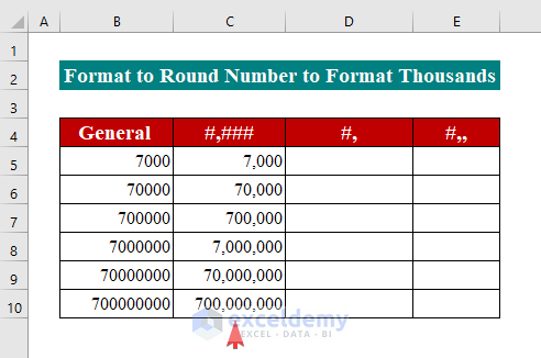
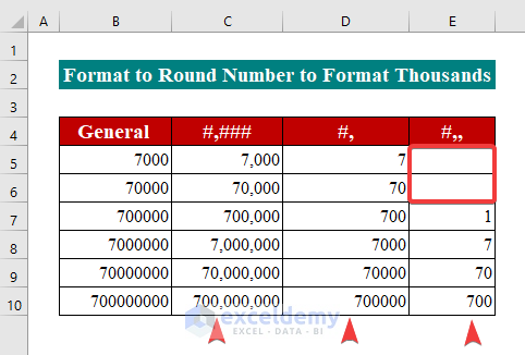
But, if there is no digit placeholder after a comma, the number is scaled by a thousand, two consecutive commas by a million, and so on.
- Select the source data and press Ctrl + 1.
- Select Custom from the Category section in the Format Cells.
- In the Type field of the Format Cell dialog box:
- For thousands, use
#, - For millions, use
#,,
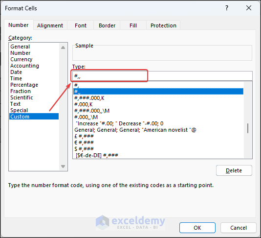
- For thousands, use
- Click OK.
- Here’s a result that shows how formatting affects the numbers.
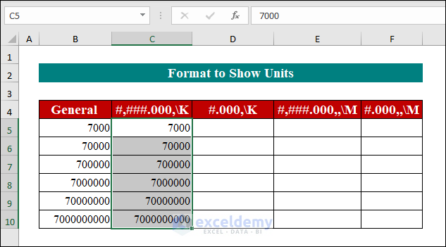
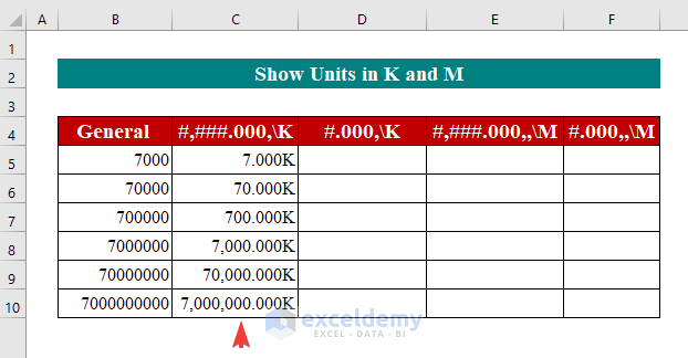
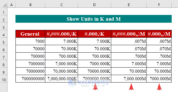
Example 4 – Adding Units with Custom Cell Formatting
The numbers can be scaled by units such as thousands and millions. Additionally, K and M can be added to the format codes.
- Select cells for which you want to apply a custom format.
- Press Ctrl + 1 to open the Format Cells dialog box.
- In the Format Cells dialog box:
- Select Custom from the Category section.
- In the Type field, use the format code:
#,###.000\K - Hit OK.
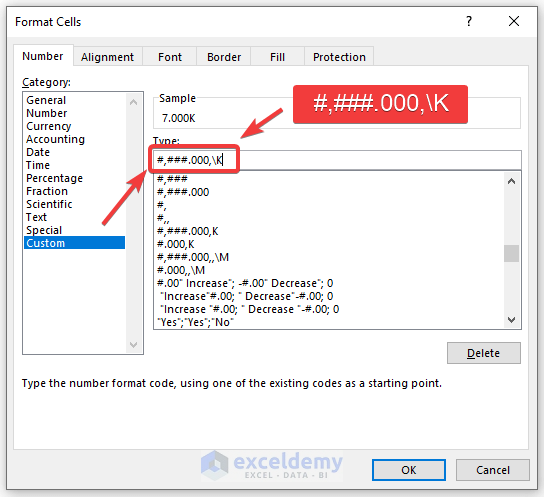
- You will see an output like the following image.
- You can repeat the steps for applying other formats.
Read More: How to Add Text after Number with Custom Format in Excel
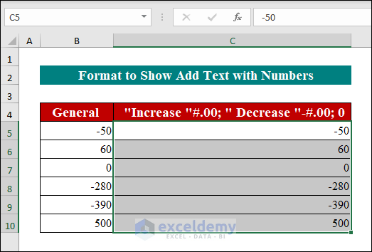
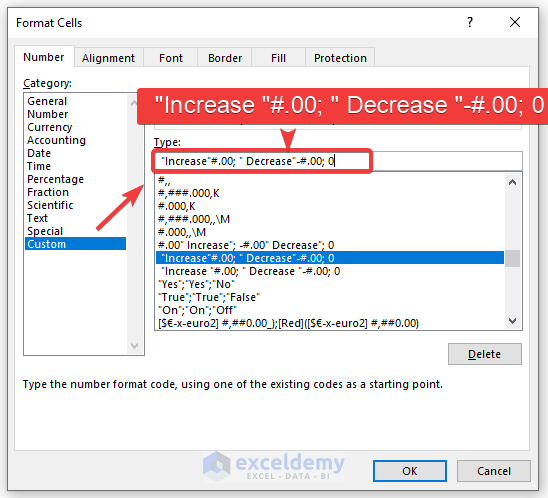
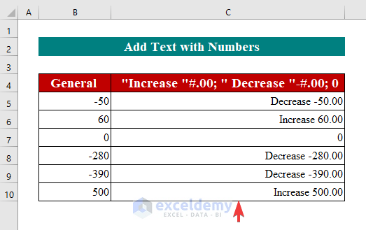
Example 5 – Adding Text in Numbers with a Custom Format
You can also show text and numbers in a single cell. For positive numbers, add the phrases “increase” and “decrease”; for negative values, add the words “decrease.” Double-quote the content in the relevant section of your format code.
- Select cells for which you want to apply a custom format code.
- Press Ctrl + 1 to open the Format Cells dialog box.
- In the Format Cells dialog box:
- Select Custom from the Category section.
- In the Type field, use the format code:
#.00" Increase"; -#.00" Decrease"; 0 - Hit OK.
- You will see the newly created format in your desired cells.
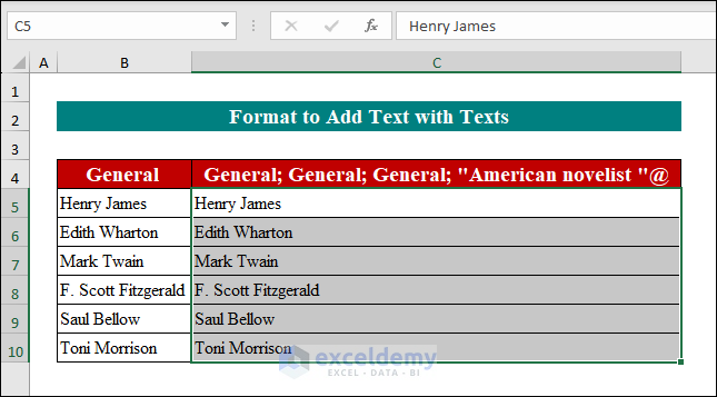
Example 6 – Adding Text Within Text in Excel Cells
You can combine some specific text with text typed in a cell by inserting the additional text in double quotes before or after the text placeholder @ in the fourth part of the format code.
- Select cells for which you want to create custom formatting.
- Press Ctrl + 1 to open the Format Cells dialog box.
- In the Format Cells dialog box:
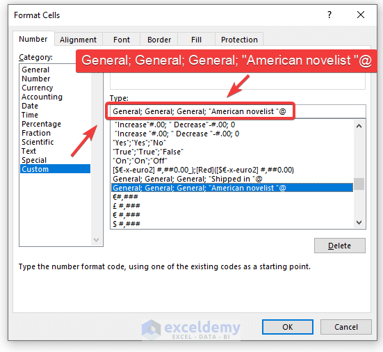
- Select Custom Under the Category section.
- In the Type box, use the format code:
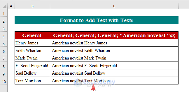
General; General; General; "American novelist "@ - Click OK.
- Here’s the effect of the format code.
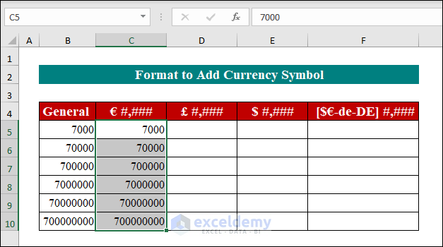
Example 7 – Displaying the Currency Symbol in Cells
You can insert the dollar symbol ($) in the relevant format code to make a unique number format. The format $#.00 will display 7000 as $7000.00. On most common keyboards, there are no additional currency symbols available. However, you can include a currency symbol by turning the NUM LOCK on and then typing the ANSI code using the numeric keypad.
| Symbols | Names | Codes |
| € (EUR) | Euro | ALT+0128 |
| ¢ | Cent Symbol | ALT+0162 |
| ¥ (JP¥) | Japanese Yen | ALT+0165 |
| £ (Sterling) | British Pound | ALT+0163 |
- Select cells for which you want to create custom formatting.
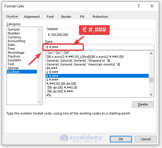
- Press Ctrl + 1 to open the Format Cells dialog box.
- In the Format Cells dialog box:
- Under Category, select Custom.
- Press NUM LOCK.
- In the Type field, use the format code:
€ #,###
To insert the € sign, press Alt + 0128.
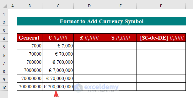
- Click OK.
- You will see that the (€) sign is added in the selected cells.
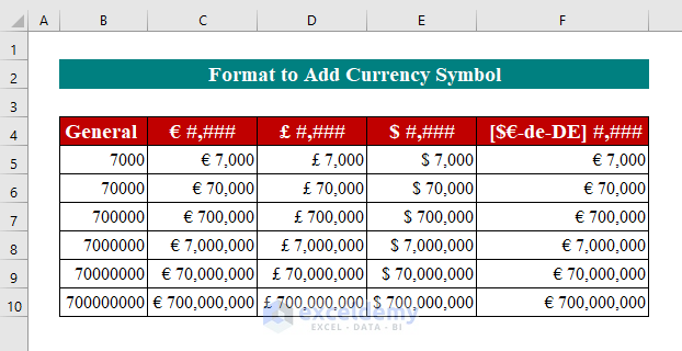
- You can repeat the steps and insert different format codes to display different currency formats.
Note: Other unique symbols, such as copyright and trademark, can be accepted in a specific Excel number format. These characters can be typed in with the Alt ANSI code.
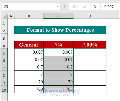
Example 8 – Displaying Percentages with a Custom Format
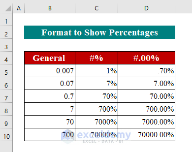
To present percentages as integers, you must first convert them to decimals. The format code will be #%. If you want to show percentages with two decimal points, use #.00% as the format code.
- Select the range for which you want to create custom formatting.
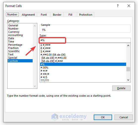
- Press Ctrl + 1 to open the Format Cells dialog box.
- In the Format Cells dialog box:
- Select Custom from the Category section.
- Use this format code in the Type field:
#% - Click OK.
- You will see the intended output like the following.
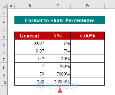
- You can repeat the steps for the rest of the ranges to get the result.
Read More: How to Format Number to Millions in Excel
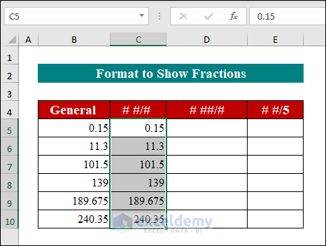
Example 9 – Converting Decimal Numbers into Fractions
Numbers can be written as mixed fractions, like 11 1/3. The custom codes you can apply for mixed fractions:
- # #/# –presents a fraction remaining of up to one digit,
- # ##/## – presents a fraction remaining of up to two digits,
- # #/5 to display decimal integers as fifths.
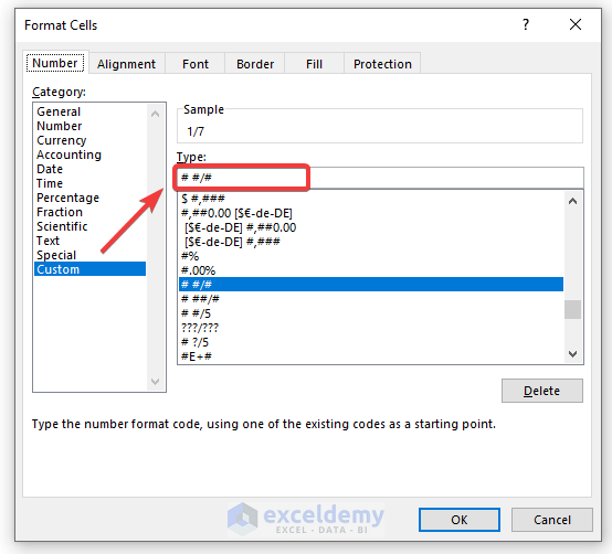
- Select cells for which you want to create custom formatting.
- Press Ctrl + 1 to open the Format Cells dialog box.
- In the Format Cells dialog box:
- Select Custom from the Category section.
- In the Type field, use the format code:
# #/# - Click OK.
- You will see mixed fractions in the selected cells.
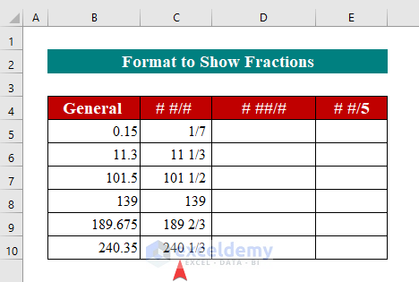
- You can repeat the steps and type different format codes like the following image.
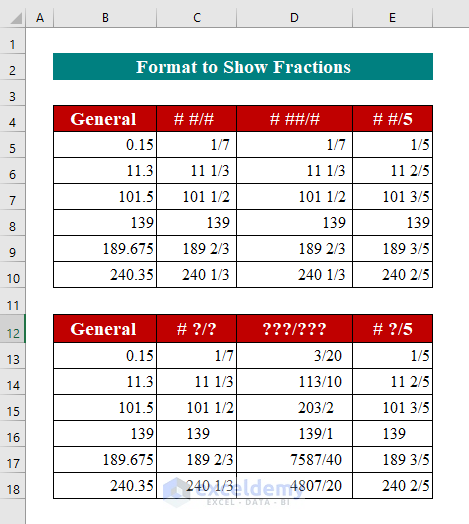
Note: Instead of the pound marks (#), you can use question mark placeholders (?) to return the number at some distance from the remainder. Add a zero and a space before the fraction in a General Cell formation to enter 5/7 in a cell—for example, type 0 5/7. When you type 5/7, Excel interprets it as a date and changes the cell format.
Example 10 – Creating a Scientific Notation in Excel Cells
You can insert the block letter E in your number format code if you want to display numbers in Scientific Notation.
- Select the desired cells for creating scientific notation.
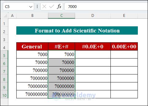
- Open the Format Cells dialog box by pressing Ctrl + 1.
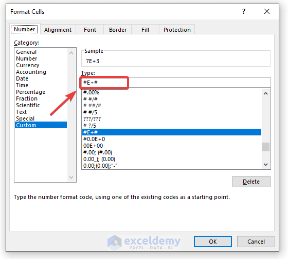
- In the Format Cells dialog box:
- Select Custom from the Category section.
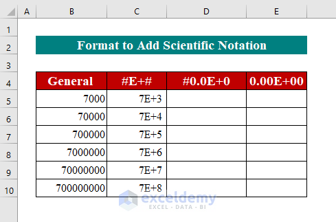
- In the Type field, use the format code:
#E+# - Click OK.
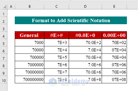
- You will see scientific notation is applied within the selected cells.
- Repeat the same steps for other notations to get the output, like the following.
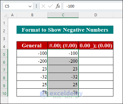
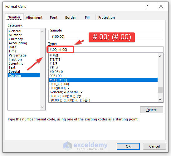
Example 11 – Showing Negative Numbers with a Custom Format
- Select cells for which you want to create custom formatting.
- Press Ctrl + 1 to open the Format Cells dialog box.
- In the Format Cells dialog box:
- Select Custom from the Category.
- In the Type field, insert the format code:
#.00; (#.00) - Click OK.
- You will see that the selected cells have new formatting, like the following image.
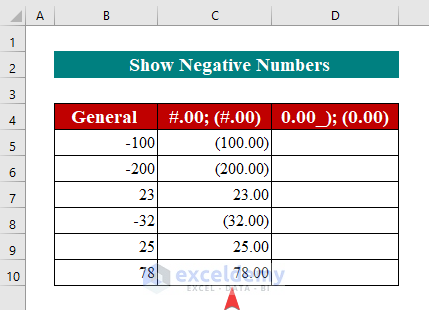
- You can follow the same steps and type different format codes for other columns.
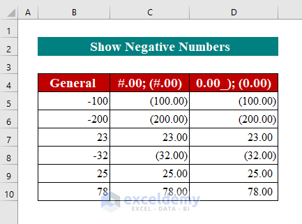
Note: Add an indent in the positive values section to align positive and negative integers at the decimal point: 0.00_); (0.00).
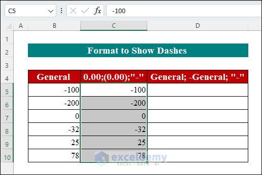
Example 12 – Displaying Dashes with a Custom Format
Zeros are displayed as dashes in accounting format.
- Select cells for which you want to create custom formatting.
- Press Ctrl + 1 to open the Format Cells dialog box.
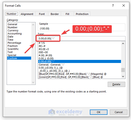
- In the Format Cells dialog box:
- In the Category section, select Custom.
- In the Type field, use the format code:
0.00;(0.00);"-" - Click OK.
- You will see the intended formatting in the selected cells.
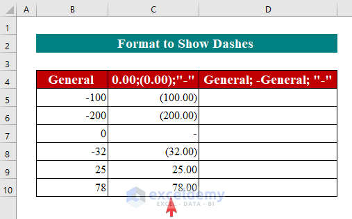
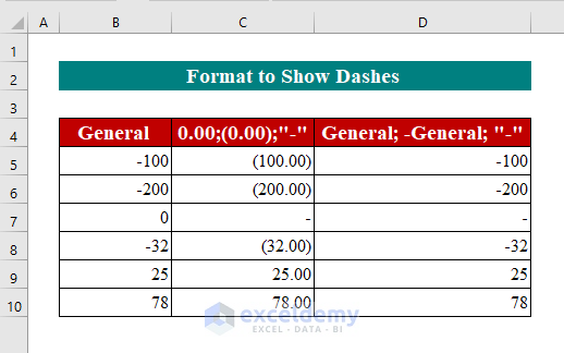
- You can follow the same steps and type different format codes to show dashes in another column.
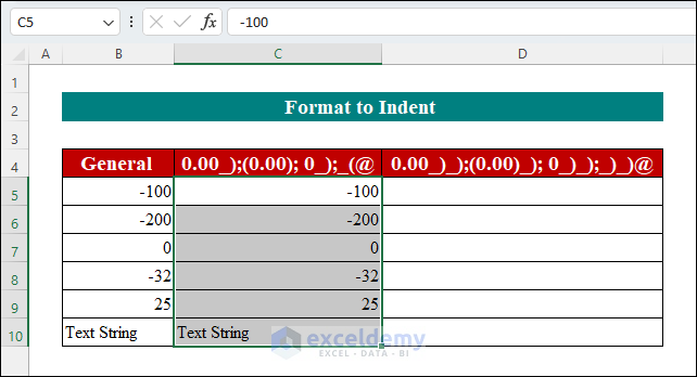
Example 13 – Including Indents with a Custom Format
Apply the underscore (_) to generate a space to add an indent. To indent from the left boundary, you can use _( and for indenting from the right boundary, use _).
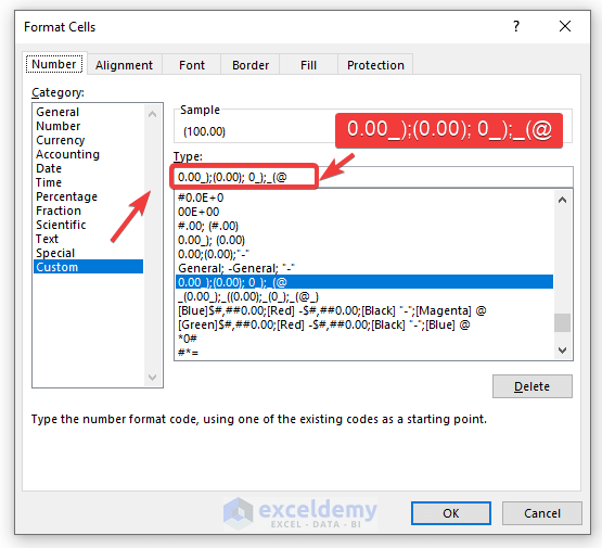
- Select cells in the range you want to create custom formatting.
- Press Ctrl + 1 to open the Format Cells dialog box.
- In the Format Cells dialog box:
- Select Custom in the Category section.
- Use this format code in the Type box:
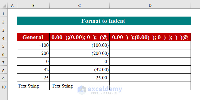
00_);(0.00); 0_);_(@ - Click OK.
- You have indented positive integers and zeros from the right and text from the left.
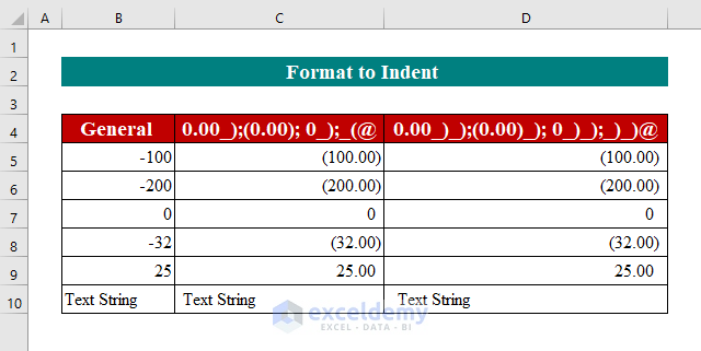
- Include two or more indent codes in a row in your custom number format to move values away from the cell borders. The picture below shows how to indent cell contents by 1 and 2 characters:
Read More: Excel Custom Number Format – Millions with One Decimal
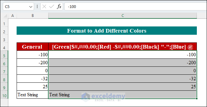
Example 14 – Adding Different Font Colors with a Custom Format
Insert [Color] before each part of the code to put it in that color.
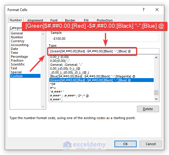
- Select cells for which you want to create custom formatting.
- To open the Format Cells dialog box, press Ctrl + 1.
- In the Format Cells dialog box:
- Select Custom from the Category section.
- Use the format code in the Type field:
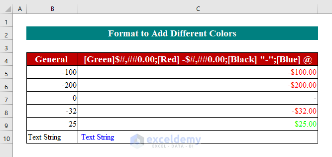
[Green]$#,##0.00;[Red] -$#,##0.00;[Black] "-";[Blue] @ - Click OK.
- You can see an output like the following image.
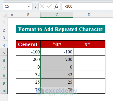
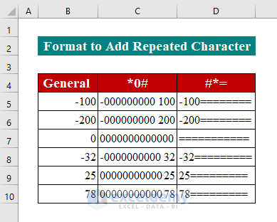
Example 15 – Repeating Characters in Excel Cells
In your bespoke Excel format, insert an asterisk * sign before the character to complete the column width with a repeated character. You can add leading zeros in any numeric format by inserting *0# before it. Or, you can use this number format to insert after a number. There are too many equality signs to occupy the cell: #*=
So, the quickest way to enter phone numbers, zip codes, or social security numbers with leading zeros is to use one of the predefined special formats. You can even construct your number format. Use this format to show international six-digit postal codes, for example, 000000. Use the following format for social security numbers with leading zeros: 000-00-000.
- Select cells for which you want to create custom formatting.
- Press Ctrl + 1 to open the Format Cells dialog box.
- In the Format Cells dialog box:
- Select Custom from the Category section.
- In the Type field, use the format code:
*0# - Click OK.
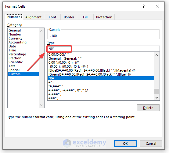
- You will see an output like the following image.
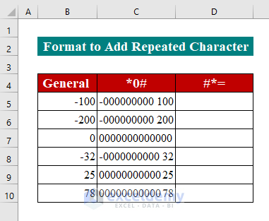
- Repeat the steps and type another format code to add repeated characters in the other column.
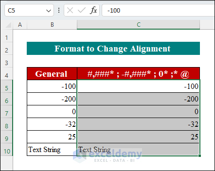
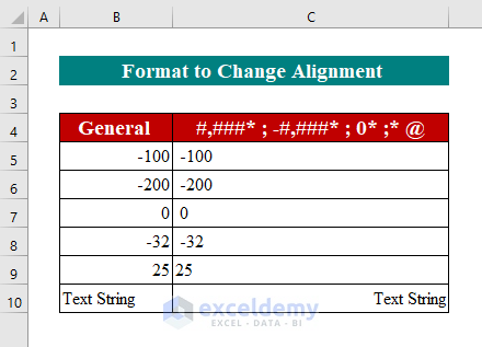
Example 16 – Changing the Alignment with Custom Format
After the number code, you can type an asterisk (*) and a space to align the numbers left in the cell; for example, “#,###* “. Taking it a step further, you can use a custom format to align numbers to the left and text inputs to the right using the following: #,###* ; -#,###* ; 0* ;* @
- Select the cells in the range in which you want to create custom formatting.
- Press Ctrl + 1 to open the Format Cells dialog box.
- In the Format Cells dialog box:
- Select Custom from the Category section.
- In the Type field, use the format code:
#,###* ; -#,###* ; 0* ;* @ - Click OK.
- You should see an output like the following image.
Read More: How to Apply Number Format in Millions with Comma in Excel
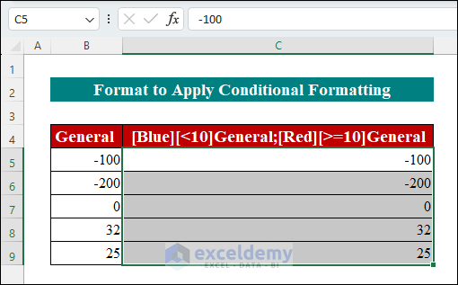
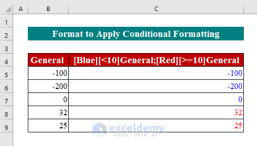
Example 17 – Applying Conditional Formatting with a Custom Format
You can also apply conditional formatting in Excel cells with the help of a custom format. You can show numbers that are less than 10 in blue and numbers that are greater than or equal to 10 in red by using the format code: [Blue][<10]General;[Red][>=10]General. The condition goes after the color code for the section.
- Select the cells in the range in which you want to create custom formatting.
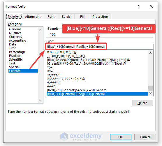
- Press Ctrl + 1 to open the Format Cells dialog box.
- In the Format Cells dialog box:
- Select Custom from the Category section.
- In the Type box, use the format code:
[Blue][<10]General;[Red][>=10]General - Click OK.
- The custom format is applied and highlights cells in the selected area.
Download the Practice Workbook
Frequently Asked Questions
How do I apply a custom temperature format in Excel?
You can use a format code like 0"°C" to apply a custom temperature format. The format code will display the temperature followed by the degree Celsius symbol (10°C).
Can VBA be used to automate custom formatting in Excel?
Yes, you can use VBA to apply custom formatting. For example, you can write a VBA script that utilizes the NumberFormat property to set custom formats for specific ranges or cells.
Related Articles
- How to Format a Number in Thousands K and Millions M in Excel
- How to Apply Custom Number Format in Excel with Multiple Conditions
- How to Add Number with Text in Excel Cell with Custom Format
<< Go Back to Custom Number Format | Number Format | Learn Excel
Get FREE Advanced Excel Exercises with Solutions!

Great article and excellent guide, keep up the good work!
Thank you MOE, for your generous appreciation!
I have a question though, can I create a custom format that rounds numbers less than a million to #, /K and numbers above a million to #,, /M ?
Thanks
Thank you MOE for your wonderful question. To do this you need to apply the following Custom Cell Format.
It would be nice to include a section on locale, either the “obsolete” LCID, such as
[$-409] – where 409 is really just hex for 1033
or the locale name
[$-en-US]
which I believe is the preferred method now.
The [$…..] notation allows for provisioning the currency symbol as well, so
[$USD -en-US]
will show $2,750.22 AS USD 2,750.22
Finding anything like Microsoft documentation on this field is very difficult, so I’m certain at least somebody finding your page would be thinking about this section of the custom format.
Hello ERFLING,
Thanks for your valuable suggestion. But you can take a look at Section 7 of this article which may align with this requirement.
Thanks
Tanjima Hossain
ExcelDemy
Hi, great stuff!
How can I create a format that has a decimal with 2 spaces if content has decimal digits, and no decimal separator if it’s an integer?
Basically #.00 if has decimals, and # otherwise.
The closest I get is #.##, but that wont give me 2 spaces of decimals if there only is one (so I’d like to fill it out with a 0 in that case), and integers will have just the decimal dot at the end which looks terrible.
Thank you, Fred, for your wonderful question.
Firstly, go to the Home tab.
You can keep the decimal places of any number at any place by using the Increase Decimal and the Decrease Decimal icons here.
Bishawajit, on behalf of ExcelDemy
Hi
When I write $#,### in the custom section I get the following result $1000000. How do I get a result that would show $1,000,000. Windows was set up in French. I wonder if that is the problem.
Thank you for your help.
Gilles
Thank you, Gilles Laurence, for your comment. I am replying on behalf of ExcelDemy. The custom number format works perfectly on our end. The French number system uses a comma for a decimal separator and a space for thousand separators. You can change the thousand separators from the Advanced tab on the Excel Options to solve this.
I would like excel to always return 8 Alpha numeric with a fill of 0 on the left side of the data string.
e.g.
1111A -> 0001111A
11111A -> 0011111A
1B -> 0000001B
Anyone can help me? I knowhow to do it with a formula =right(“0000000″&A1,8). This will require me using a separate cell. I would like the modification to happen in the original cell itself. I am sure the Excel has this function I just cant figure it out.
Thanks for any help.
Hi KARL,
Thanks for your comment.
To always return 8 digits with a fill of 0 on the left side of the data you can use VBA code. Follow the steps given below to do that.
Steps:
• Firstly, go to the Developer tab >> click on Visual Basic.
• Then, it will open Microsoft Visual Basic for Applications.
• Now, open Insert >> select Module.
• Next, a Module will open then type the following code in the opened Module.
• Finally, Save the code and go back to the worksheet.
• Then, select the cell or cell range to apply the VBA.
• Here, we selected the range B5:B7.
• Next, open the Developer tab >> select Macros.
• After that, select Alphanumeric and click on Run.
• Thus, Excel will always return 8 Alphanumerics with a fill of 0 on the left side of the data string.
We hope this will solve your problem. Please let us know if you face any further problems.
Regards,
Arin Islam,
ExcelDemy
Thank You!
Hello, JeteMc!
Welcome, JeteMc. To get more helpful information stay in touch with ExcelDemy.
Regards
ExcelDemy
How to show 100 in value 25=100/4 by using formula custom cell format , without change the original value
Dear Deepak,
Thank you for your comment.
To show 100 in value 25=100/4, you need to apply the following Custom Cell Format.
Best,
Afia Aziz Kona
Can I set negative numbers color with hex (ie ‘#FF6600’) instead of the name of the color (ie ‘[RED]’)?
Best,
Anton
Dear Anton!
Thanks for reaching out and sharing your problem with us.
No, you can not set the color of negative numbers using hex values directly in the custom number format in Excel. The custom number format in Excel has predefined color names such as [Red], [Green], etc., but it doesn’t support specifying colors using hex values.
Again, thank you for being with us.
Regards
Md. Abdur Rahim Rasel
Exceldemy Team
I would like to know what format code I would need to use to when I want my display units in the thousands to read 0.00GW and not 0.00KGW.
When I set my display units as “none” and try to use a custom format: #.##,\GW it will read as 0,000GW or 0000GW. If I keep the display unit set to Thousands and add the custom format the data is displayed as 0.00KGW.
Hello Maddie,
To display units in thousands without “K”. You can use the format #.##,,”GW” for thousands (without “K”).
This removes the extra “K” while formatting the number in thousands.
Regards
ExcelDemy
This format does not remove the “K” for me. Instead, it keeps the “K” and now the numbers/values are removed.
Hello Maddie,
It seems the custom number format you’re using might be interacting with the display unit settings in Excel.
Set the display units to “None”. Display units in Excel (e.g., “Thousands”, “Millions”) automatically append prefixes like “K” or “M”, and in this case, that’s why the “K” is appearing.
Use this custom format: 0.00,, “GW” or #.##,,”GW”
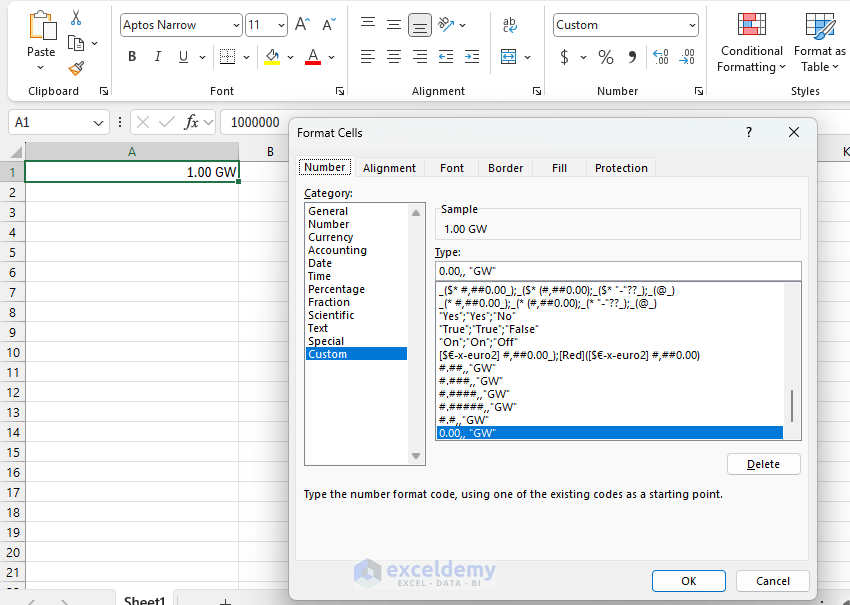
The double commas ,, divide the number by 1,000 twice, which effectively formats the number in thousands. The result should display values in thousands with “GW” as the unit but without adding “K”.
By setting the display units to “None” and using the format above, the unwanted “K” should no longer appear, and the values will remain visible.
Regards
ExcelDemy
Hi, i have an issue i hope you can help me with, i have some dates that are treated internally as texts and are shown in the format 13.01.2000, wich, for the most part is fine, but when the date is null, it shows 00.00.0000, i would like to change it so that it would either show something else (like a “#”), or change color so it can’t be seen. Can this be done with the Custom format cell or am i barking at the wrong tree?, also, i cannot do this with the condittional formatting option bc my table is dynamic
Hello Santiago,
You can handle this by using a custom cell format. To replace 00.00.0000 with a placeholder (like #) or hide it, try using this custom format: dd.mm.yyyy;@;.
You can add ; after each section to control how positive, negative, zero, and text values display, respectively.
For example, dd.mm.yyyy;@;#;”” will show # for zero values. Custom formatting, however, only changes the display, not the underlying data.
Regards
ExcelDemy
Thank you very much for your answer before, i also wanted to ask if it is possible to change the background color of the cell with the Custom format Cell. As always, thank you very much, and i hope you have a great day.
Hello Santiago,
You’re welcome! Unfortunately, custom cell formats in Excel only change the appearance of the data (like number format or text display) and cannot modify the background color of a cell.
To change the background color based on certain criteria, you would need to use Conditional Formatting. Although your table is dynamic, you can apply conditional formatting rules that automatically adjust to new data. For example, you could set a rule to change the background color when the cell value is 00.00.0000.
Let me know if you’d like help setting that up. Have a wonderful day!
Best regards,
ExcelDemy