How to Format Excel Values as Millions with One Decimal Place (6 Methods)

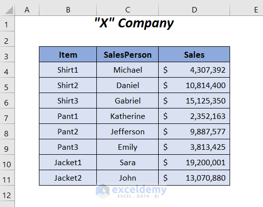
Scenario

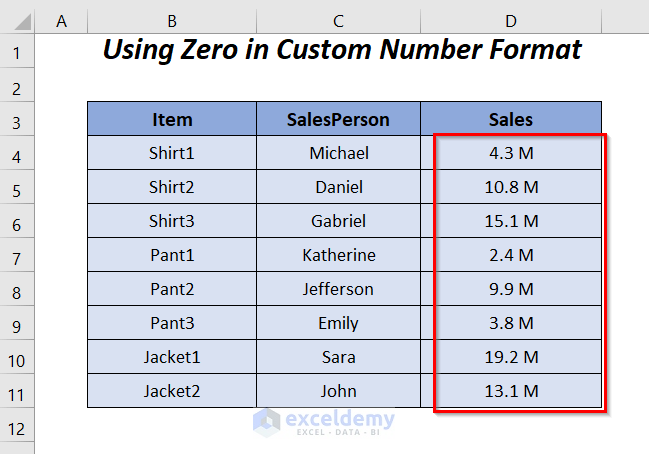
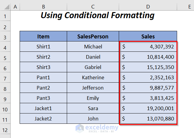
Suppose we have a dataset with large sales values that are cumbersome to read quickly. We want to use a custom number format to display these values in millions with one decimal place. Additionally, we’ll explore different methods to achieve this.

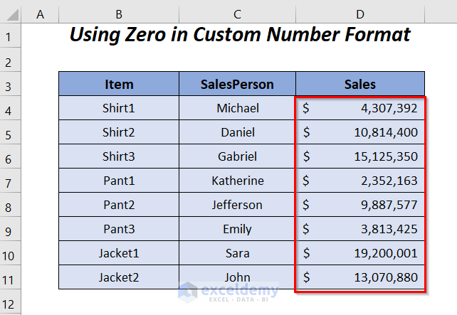
Method 1 – Custom Number Format with Zero (0)

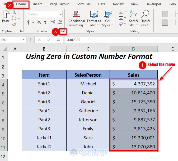
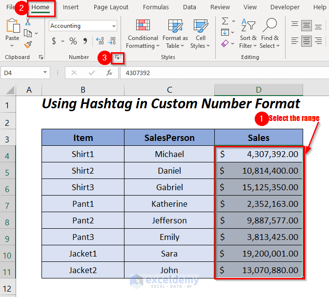
• Select the range of cells containing the sales values.
• Go to the Home tab, navigate to the Number group, and click on the Number Format dialog box symbol. Alternatively, you can press CTRL+1.

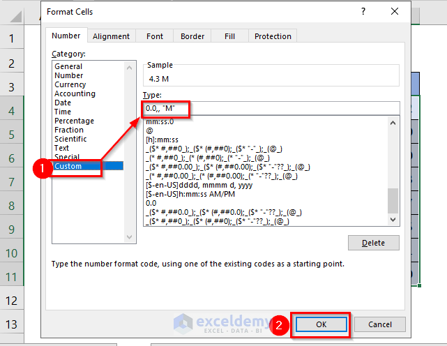
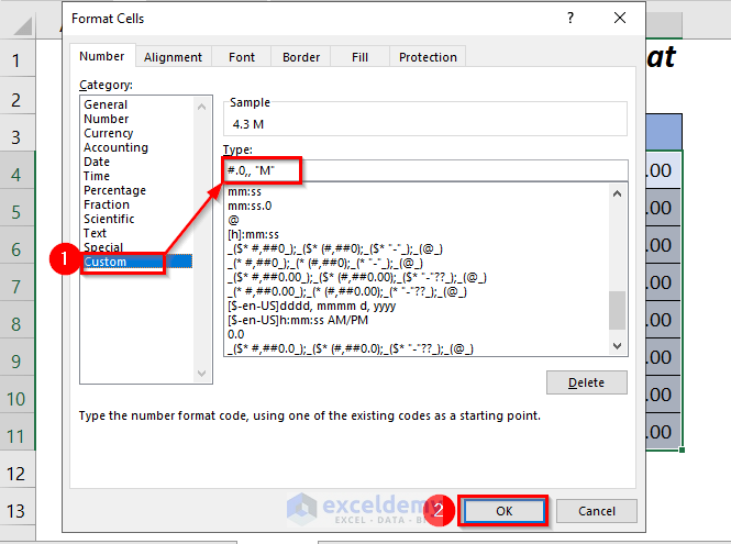
• The Format Cells dialog box will appear.
• Click on the Custom category and enter the following format in the Type box:

The 0 represents the numeric part of the value.

The two commas represent millions (since the million value has two commas 1,000,000).

The “M” is the suffix we want to add after the value to indicate millions.

• Press OK.

The sales values will now display in the desired format, with one decimal place and the “M” indicator. These values remain in number format, allowing you to perform calculations.

Read More: How to Custom Number Format in Excel with Multiple Conditions

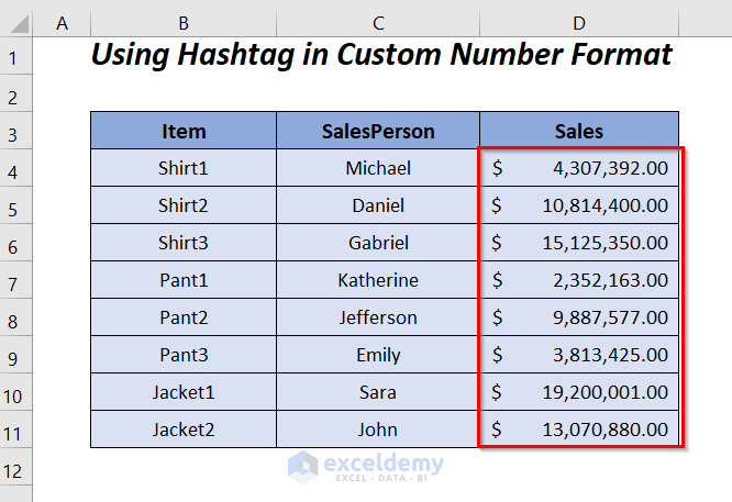
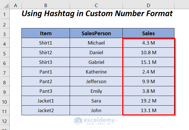
Method 2 – Hashtag Symbol (#) in Custom Number Format

• Select the range of cells containing the sales values.
• Go to the Home tab, navigate to the Number group, and click on the Number Format dialog box symbol.

• The Format Cells dialog box will open.
• Click on the Custom category and enter the following format in the Type box:

• • The # serves as a placeholder for any numeric value before the decimal point.
  • The 0 is used after the decimal point. If a value has no decimal part, it will display as zero (e.g., 1.0 M).
  • The two commas represent millions.
  • The “M” suffix indicates millions.

• Press OK.

You’ll now have sales values formatted as millions with one decimal place, and these values will be stored as numbers.

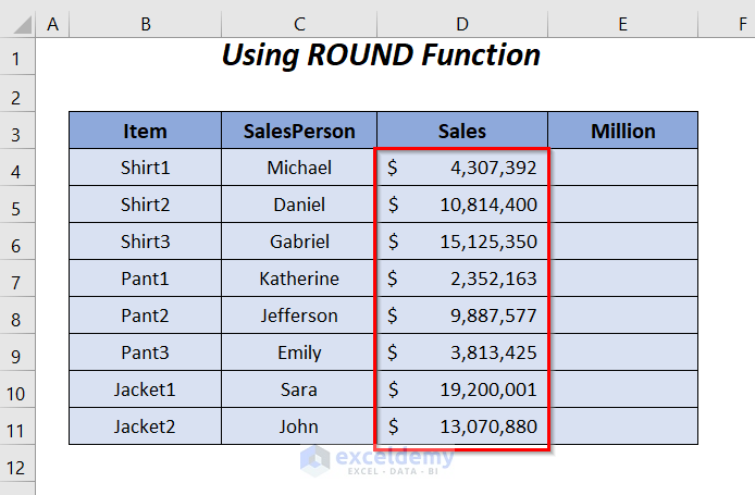
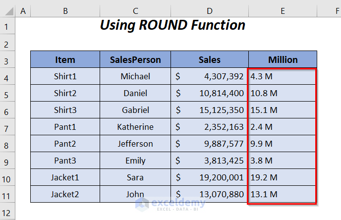
Method-3 – Using the ROUND Function to Format Sales Values as Millions with One Decimal

In this section, we’ll leverage the ROUND function along with the Ampersand operator to change the format of large sales values to millions with one decimal place.

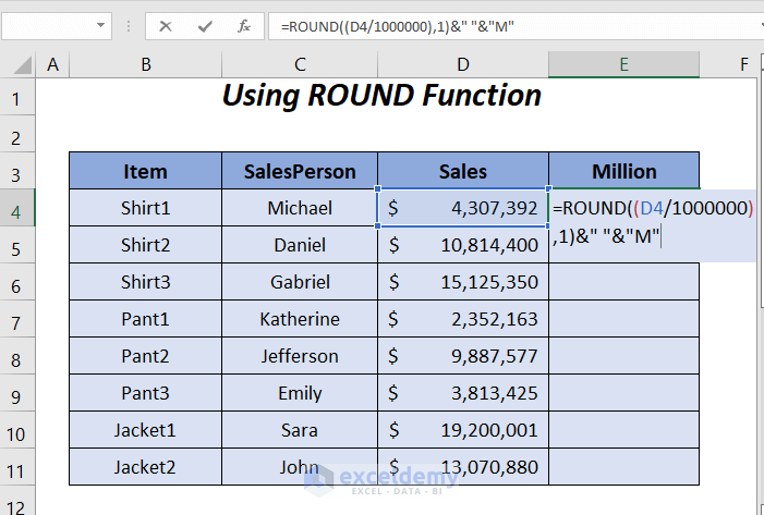
• Enter the following formula in cell E4:

• • Here, D4 represents the sales value.
  • D4/1000000 calculates the value divided by 1,000,000.
  • The ROUND function rounds the result to one decimal place.
  • The Ampersand (&) joins the rounded value with a space and the suffix “M.”

• Press ENTER and drag down the Fill Handle tool.

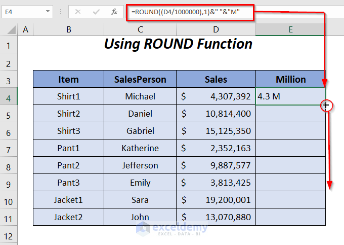
As a result, the sales values will be displayed in the desired format (e.g., 4.3 M), but they will be treated as text (not numbers) for calculations.

Read More: How to Format Number to Millions in Excel

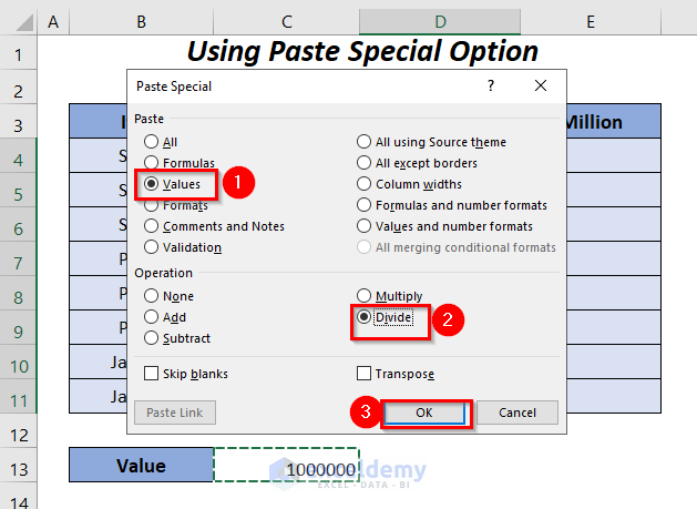
Method 4 – Using the Paste Special Option for Millions with One decimal

To execute the Paste Special option, we need the value 1,000,000 (since 1M = 1,000,000). Follow these steps:

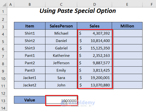
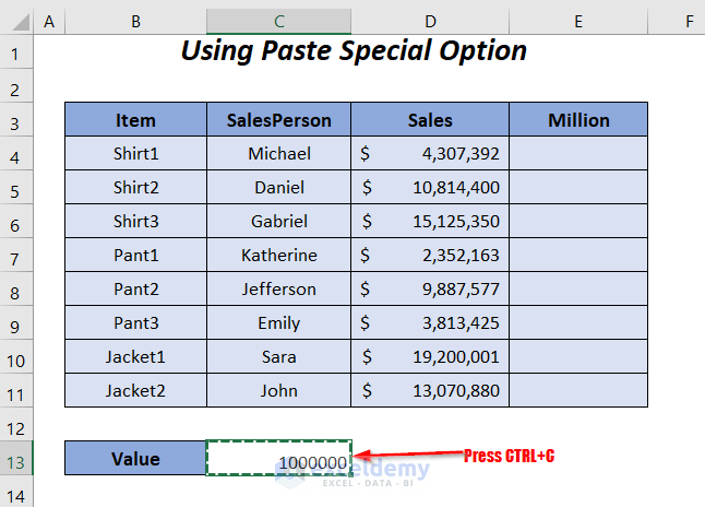
• Choose the value of cell C13 and press CTRL+C.

• Select the range of the Sales column, right-click, and choose the Paste Special option.
  • Alternatively, use the shortcut key ALT + E, S (press ALT and E together, then S).

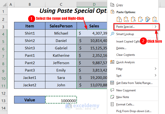
• In the Paste Special wizard, select the options Values and Divide, then press OK.

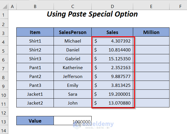
The sales values will now be divided by 1,000,000, resulting in fractional numbers. To display them as millions with one decimal place, follow these additional steps:

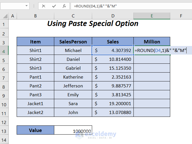
• Enter the following formula in cell E4

• • D4 represents the fraction sales value.
  • The ROUND function rounds it to one decimal place.
  • The Ampersand (&) adds the suffix M after a space.

• Press ENTER and drag down the Fill Handle tool.

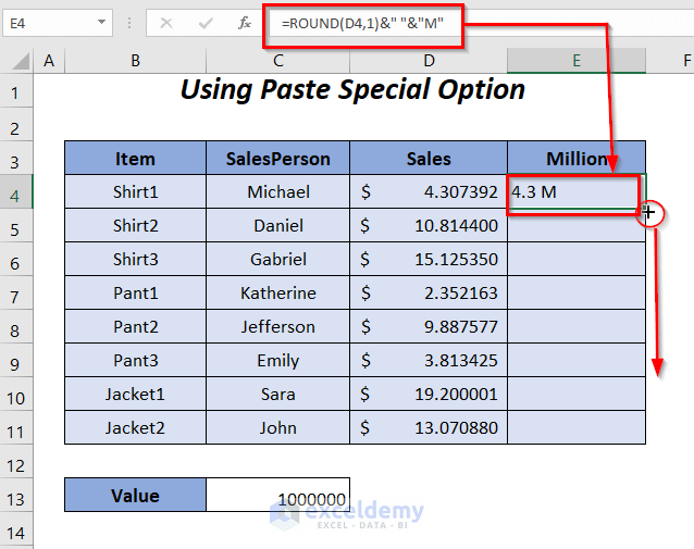
The formatted sales values will be stored as text (not numbers).

Read More: How to Format a Number in Thousands K and Millions M in Excel

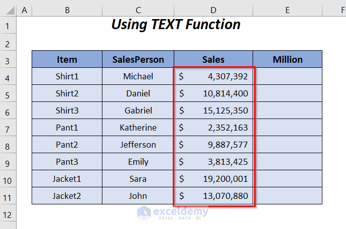
Method 5 – Using the TEXT Function for Millions with One Decimal in Excel

In this section, we’ll use the TEXT function to change the format of sales values to an easily readable format indicating millions with one decimal place. Keep in mind that after formatting, these values won’t be usable for calculations.

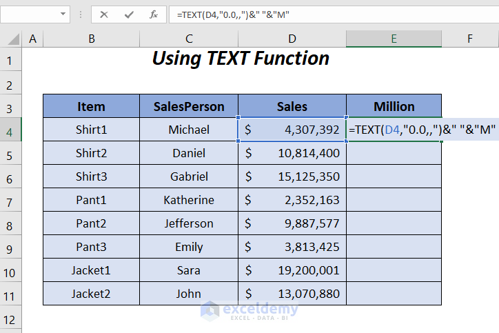
• Enter the following formula in cell E4:

• • D4 represents the sales value.
  • 0.0, specifies the formatting for millions.
  • The Ampersand (&) adds the M indicator after a space.

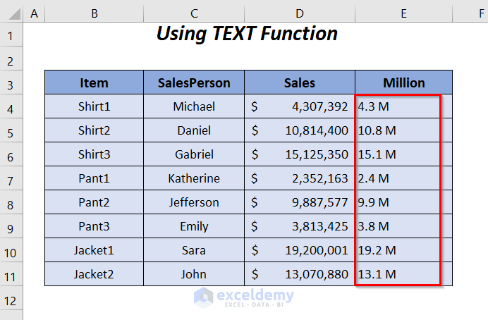
• Press ENTER and drag down the Fill Handle tool.

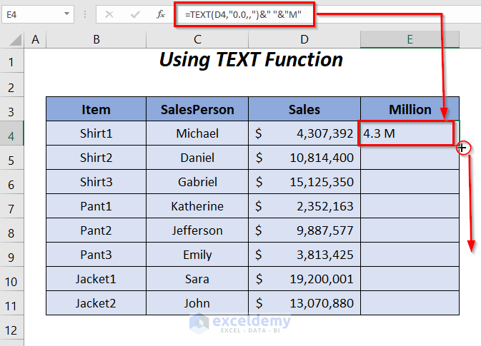
This approach will give you sales values formatted as millions with one decimal place. Remember that they’ll be stored as text.

Read More: How to Apply Number Format in Millions with Comma in Excel

Method 6 – Using Conditional Formatting for Millions with One Decimal

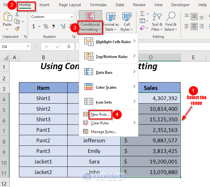
Select the Range:

• Highlight the range of cells containing the sales values that you want to format.

Access Conditional Formatting:

• Go to the Home tab.
• In the Styles group, click on the Conditional Formatting dropdown.
• Choose New Rule.

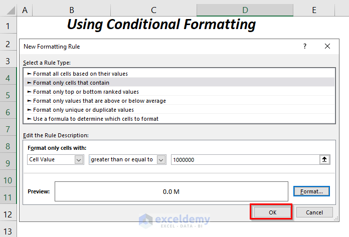
Configure the Rule:

• In the New Formatting Rule wizard, select the option “Format only cells that contain.”
• In the three input boxes, enter the following:
  • First Box: Cell Value
  • Second Box: greater than or equal to
  • Third Box: 1000000

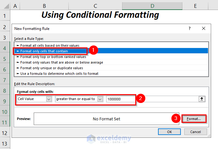
Define the Custom Format:

• After clicking the Format button, the Format Cells dialog box will appear.
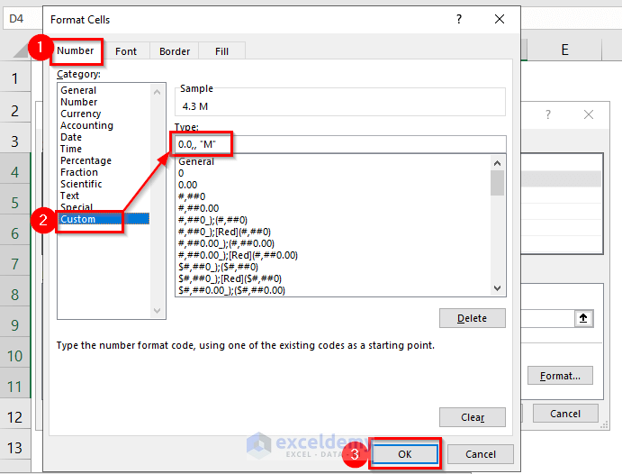
• Go to the Number tab.
• Choose the Custom category.
• In the Type box, enter the following format:

• • The 0 represents the numeric part of the value.
  • The two commas represent millions (since the million value has two commas: 1,000,000).
  • The “M” is the suffix we want to add after the value to indicate millions.

• Press OK.

Apply the Rule:

• Back in the New Formatting Rule dialog box, press OK.

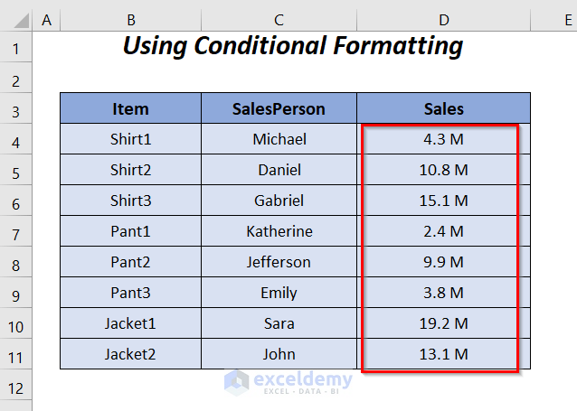
Now, your sales values will be displayed in the desired format (e.g., 4.3 M), indicating millions with one decimal place. Keep in mind that these formatted values will be stored as text (not numbers) and won’t be usable for calculations.

Read More: How to Add Number with Text in Excel Cell with a Custom Format

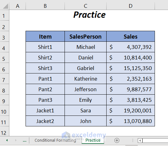
Practice Section

We have provided a Practice sheet named Practice.

Download Workbook

You can download the practice workbook from here:

Related Articles

• How to Apply Custom Format Cells in Excel
• How to Add Text after Number with Custom Format in Excel
  

<< Go Back to Custom Number Format | Number Format | Learn Excel