How to Add Number with Text in Excel Cell with Custom Format (4 Ways)

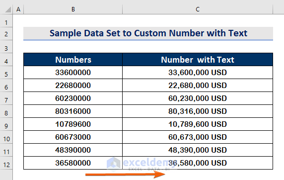
We will use four different approaches to add text with numbers to customize a cell format. Here’s a simple data set to showcase how we’ll convert numbers into text.

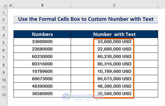
Method 1 – Using the Formal Cells Dialog Box to Create a Custom Number with Text Format in Excel

Steps:

• Select all the cells.

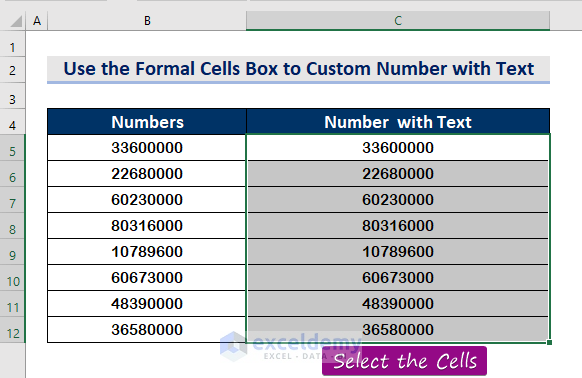
• Press Ctrl + 1 to open the Format Cells.
• Click on Custom.
• Select or type any format you need.

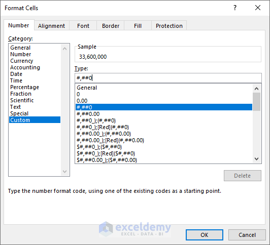
• In the Type box, write any text closed in the (“ ”). We will add USD with the following formula. #,##0 “USD”

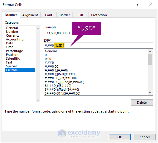
• Press Enter to get the results.

Read More:  How to Apply Custom Number Format in Excel with Multiple Conditions

Method 2 – Applying an Excel Formula with an & Operator to Create a Custom Cell Format for a Number with Text

Steps

• Select any cell.
• Put an ampersand (&).
• Type the text enclosed with the inverted comma (“USD”).
• For our sample, this will look like the following for C5: =B5&” USD”

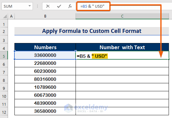
• Press Enter to see the first result.

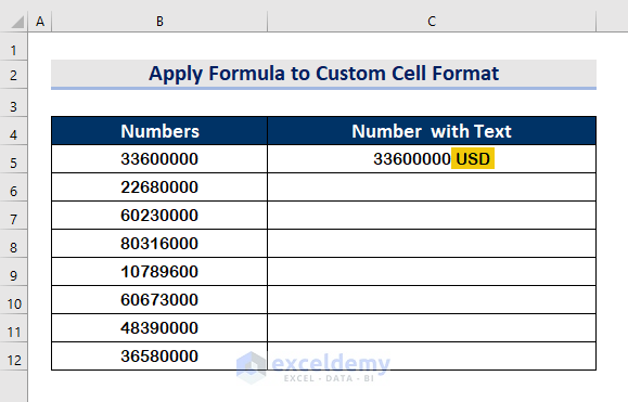
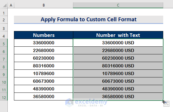
• Use AutoFill to fill up the other blank cells in the column.

Read More: How to Apply Custom Format Cells in Excel

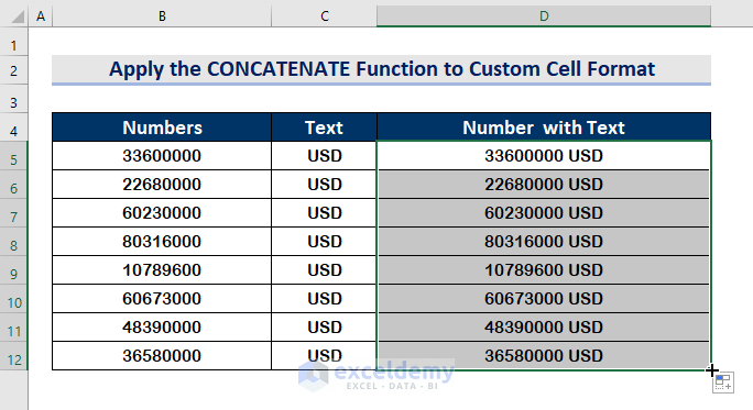
Method 3 – Inserting the Excel CONCATENATE Function for a Custom Cell Format for a Number with Text

Steps

• Use the following function in C5:

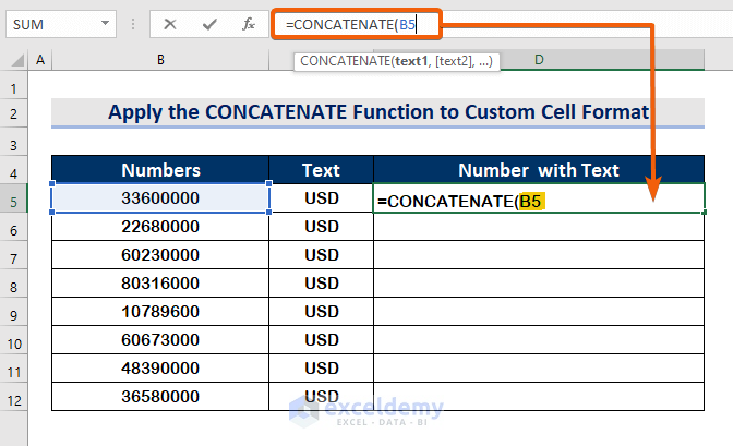
• Add a space (“ ”) for text2.

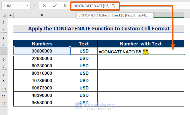
• Type any text (“USD”) as text3 with the following formula.

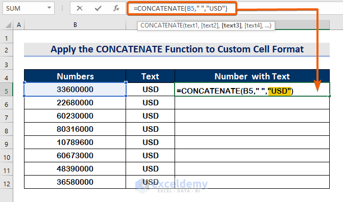
• Press Enter to obtain the result.

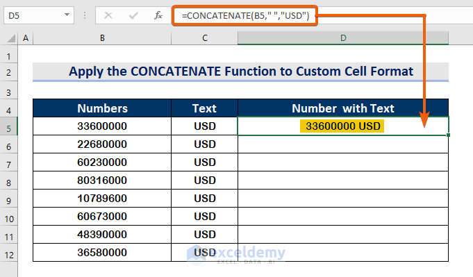
• Use AutoFill to fill in all blank cells.

Read More: Excel Custom Number Format – Millions with One Decimal

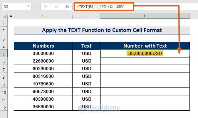
Method 4 – Applying the TEXT Function to a Custom Cell Format for a Number with Text in Excel

Steps

• Select cell D5 and put the following formula.

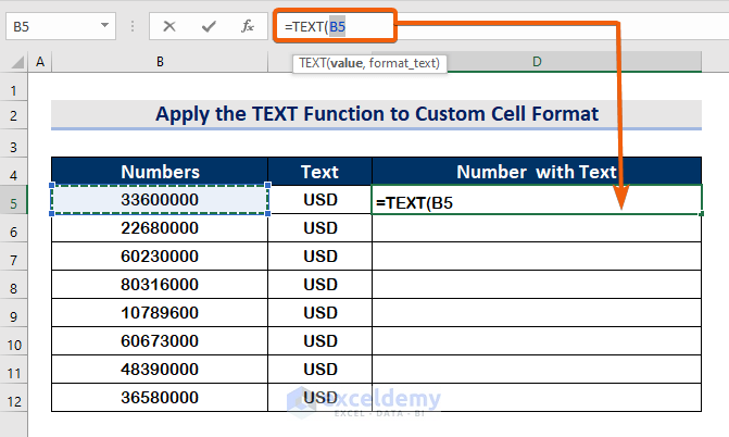
• Apply the formatting code in the function:

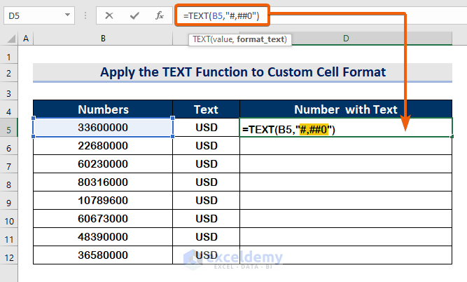
• To add text with the format cell, add any text (“USD”) with the following formula using the & operator.

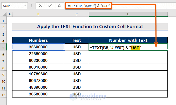
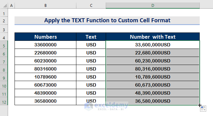
• Press Enter.

• Use AutoFill to fill all the required cells.

Read More: How to Add Text after Number with Custom Format in Excel

Download the Practice Workbook

Related Articles

• How to Format a Number in Thousands K and Millions M in Excel
• How to Apply Number Format in Millions with Comma in Excel
• How to Format Number to Millions in Excel

<< Go Back to Custom Number Format | Number Format | Learn Excel