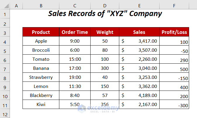
In the following dataset are the Order Time, Weight, Sales, and Profit/Loss of some products, with data in a variety of numeric formats. In this article, we’ll add text after the numbers in the different columns using a custom format, while preserving the numeric formats.
We have used Microsoft Excel 365 here, but the Methods below also apply to any other version of Excel.
Method 1 – Add Text after Numbers
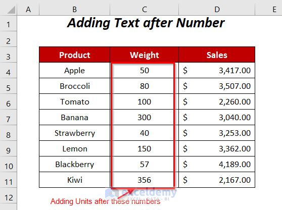
In the Weight column, let’s add the text Pound to each cell, but in such a way that the numeric values remain numeric, so that we can perform mathematical operations on them later.
Steps:
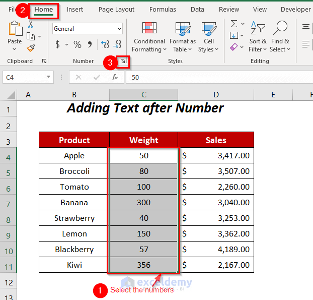
➤ Select the cells of the Weight column.
➤ Go to the Home Tab >> Number Group >> Number Format dialog box.
The Format Cells wizard will open up.
➤ Go to the Number Tab >> Custom Option >> Enter the format 00 “Pound” in the Type box.
➤ Click OK.
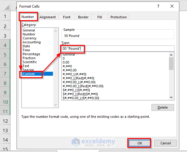
The unit Pound appears behind the weight values of the products.

Read More: How to Add Number with Text in Excel Cell with a Custom Format
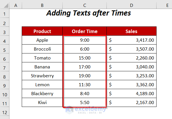
Method 2 – Add Text after Times
Now let’s change the style of the values in the Order Time column by adding AM/PM and the text string EST after the time values.
Steps:
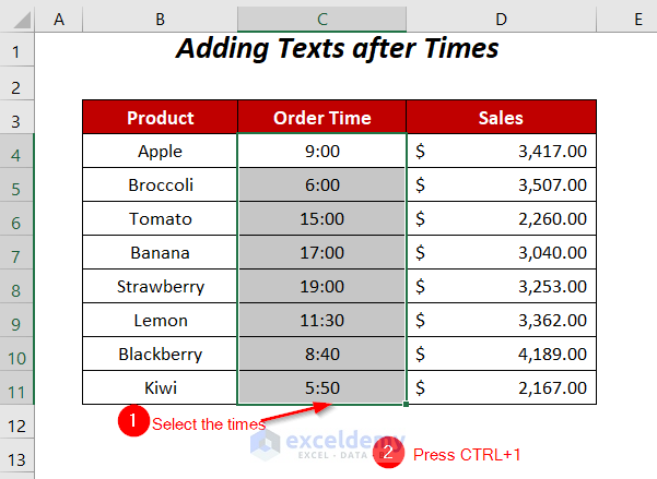
➤ Select the cells of the Order Time column.
➤ Press CTRL+1 to open up the Format Cells dialog box.
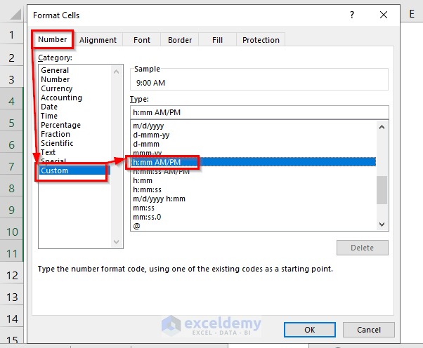
The Format Cells wizard will open up.
➤ Go to the Number Tab >> Custom Option >> Select hh: mm AM/PM from the dropdown list under the Type box.
➤ Enter the text string “EST” after the time format “hh: mm AM/PM “.
➤ Click OK.
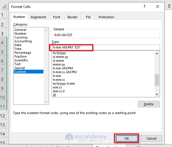
The desired time format with text EST after the time values is displayed. Numeric calculations can still be applied to these cells as before.

Read More: How to Format a Number in Thousands K and Millions M in Excel
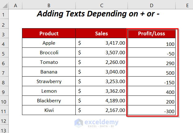
Method 3 – Add Text Depending on Positive or Negative Number
Say we have some positive values indicating the profits and negative values the losses of our products in the Profit/Loss column. Let’s add a text string Profit or Loss to these cells using a custom format.
Steps:
➤ Select the cells of the Profit/Loss column.
➤ Go to the Home Tab >> Number Group >> Number Format dialog box.
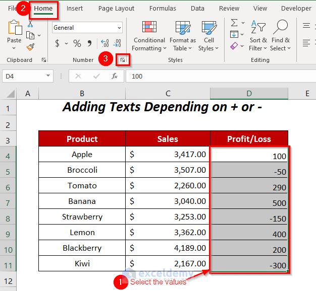
The Format Cells dialog box will appear.
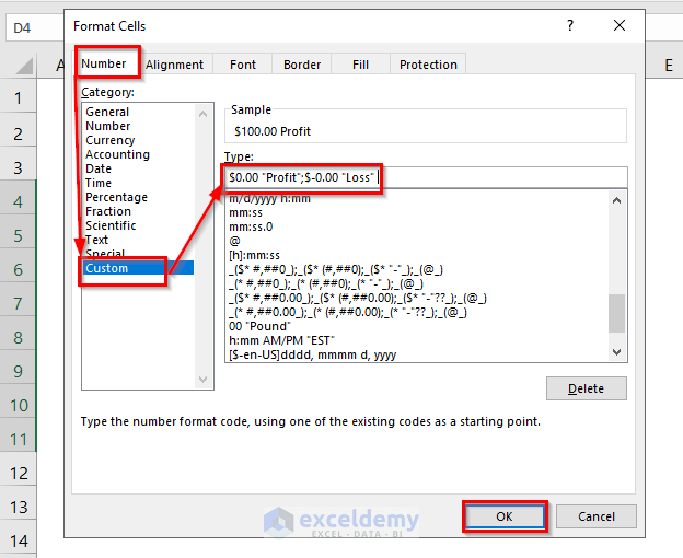
➤ Go to the Number Tab >> Custom Option >> enter the format $0.00 “Profit”;$-0.00 “Loss” in the Type box.
➤ Press OK.
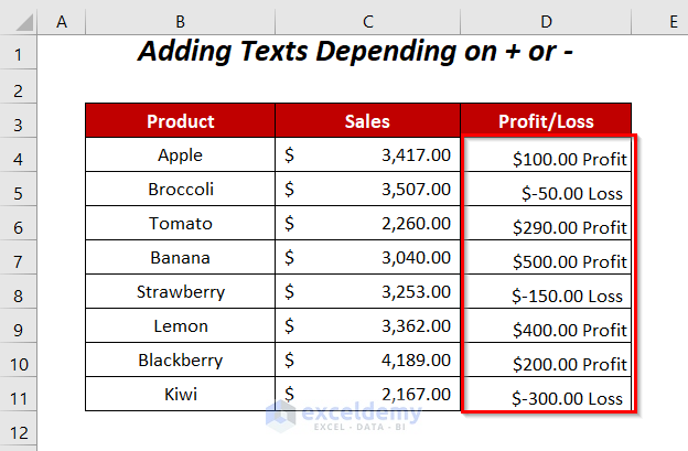
The specified text is added in the Profit/Loss column. Again, the numbers remain in numeric form, so you can sum them to calculate total Profit/Loss or perform any other calculations as before.
Read More: How to Format Numbers to Millions in Excel
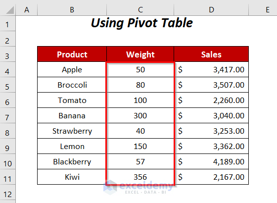
Method 4: -Add Texts after Number Using Pivot Table
Now let’s use a Pivot Table to add our desired unit Pound after the numbers in the Weight column.
Steps:
➤ Go to the Insert Tab >> PivotTable Option.
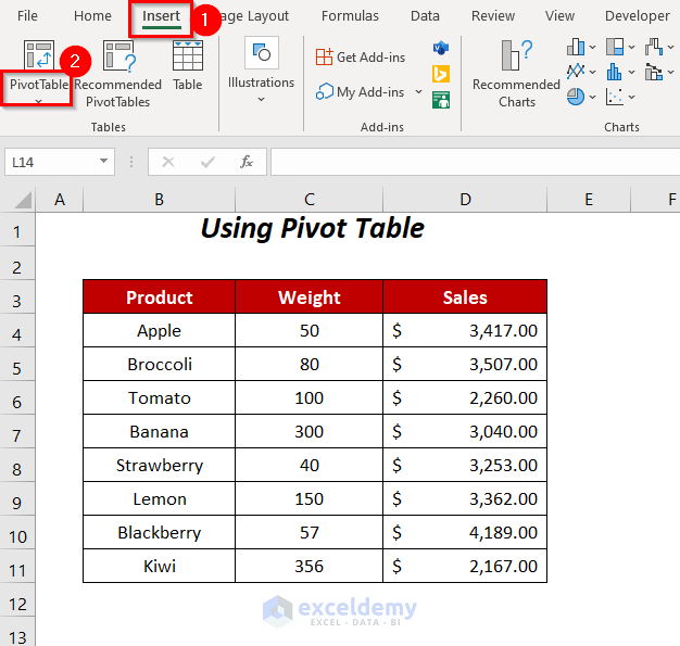
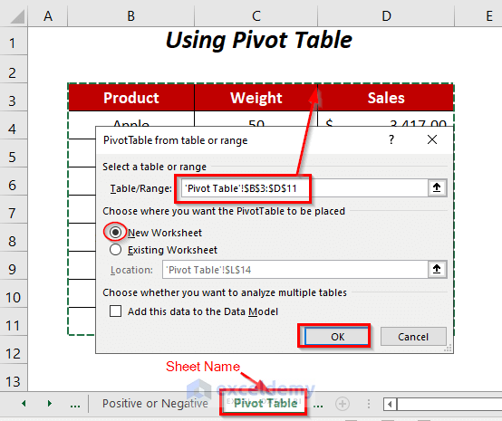
The PivotTable from table or range dialog box will pop up.
➤ Select the range of your table, and click on the New Worksheet option.
➤ Click OK.
A new sheet opens containing two parts: PivotTable1 on the left side and PivotTable Fields on the right side.
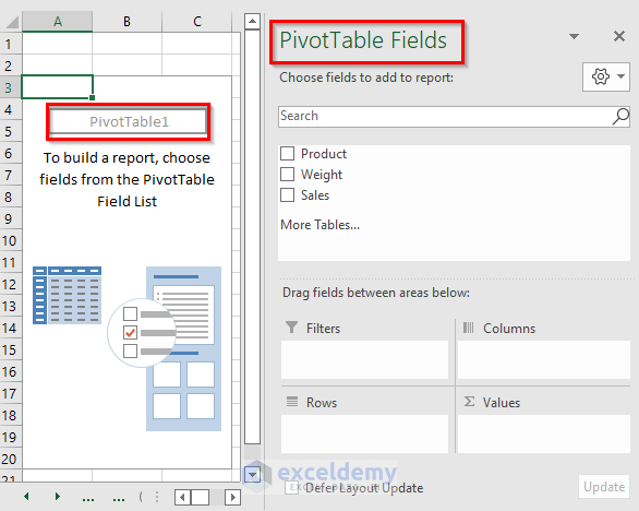
➤ Drag down the Product and Weight fields to the Rows area and Values area respectively.
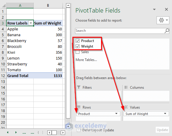
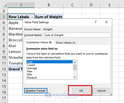
➤ To add our custom format to the weights, after clicking the dropdown symbol beside the Sum of Weight, select the Value Field Settings option from the list.
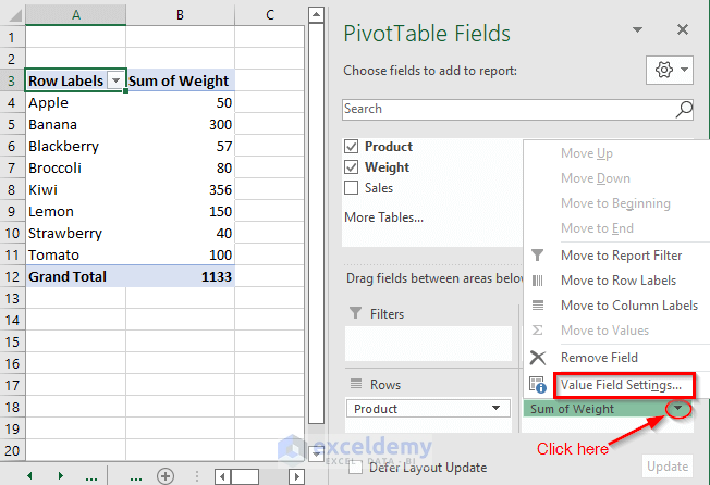
The Value Field Settings wizard will open up.
➤ Click Number Format.
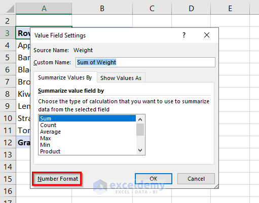
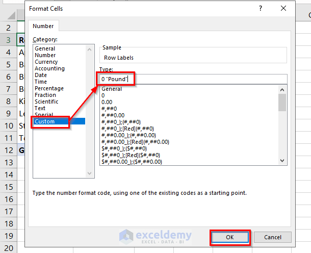
The Format Cells dialog box will appear.
➤ Go to the Custom Option >> Enter the format 0 “Pound” in the Type box.
➤ Press OK.
➤ Click on OK in the Value Field Settings dialog box.
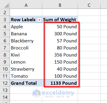
The values in the Pivot Table now include the word Pound, while remaining in numeric format.
Adding Text after a Number Without Preserving Numeric Formats
There are also several ways to add text after a number in Excel where the output will be a text format rather than numeric like in the examples above.
Let’s use the CONCATENATE function to add the unit Pound to the numeric values in the Weight column.
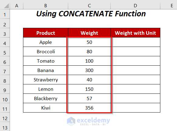
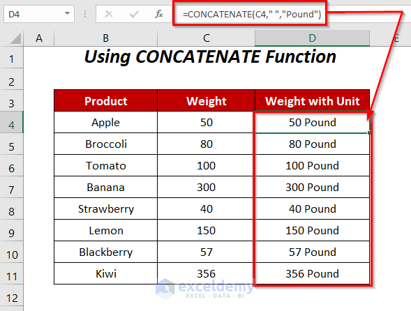
➤ In cell D4, enter the following formula:
=CONCATENATE(C4," ","Pound")➤ Use the Fill Handle to drag the formula down the rest of the column.
Here, C4 is the weight value, and CONCATENATE will combine it with the text string “Pound” with a separator of a space.
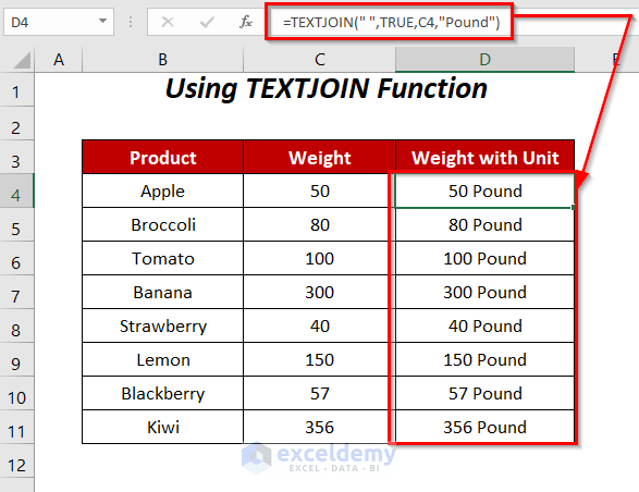
The following formula will also join numbers and text:
=TEXTJOIN(" ",TRUE,C4,"Pound")Here, C4 is the weight value and the TEXTJOIN function will combine it with the text string “Pound” with a separator of a blank.
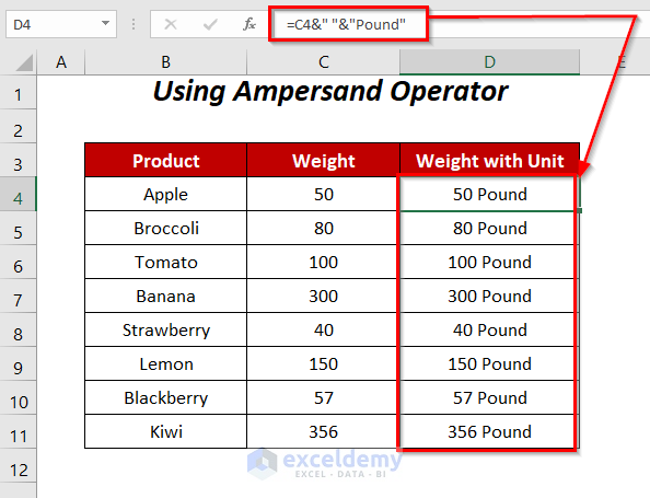
The Ampersand operator will perform the same operation as the previous two functions:
=C4&" "&"Pound"Here, C4 is the weight value, & will join this value with the text string Pound separated by a blank.
We can also add text to a number depending on whether it’s positive or negative (as in Method 3 above) by using the IF function in conjunction with the TEXT function.
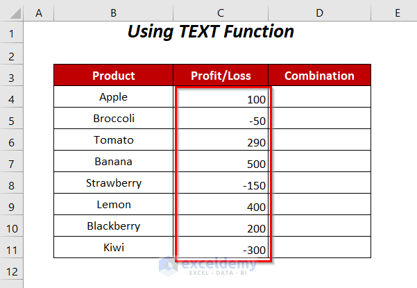
➤ Enter the following formula in cell D4:
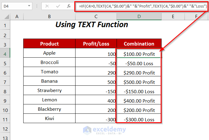
=IF(C4>0,TEXT(C4,"$0.00")&" "&"Profit",TEXT(C4,"$0.00")&" "&"Loss")Here, C4 is the weight value.
- TEXT(C4,”$0.00″) → gives the format to the value in cell C4
Output → $100.00
- TEXT(C4,”$0.00″)&” “&”Profit” becomes
$100.00 &” “&”Profit” → & operator will join the amount with the text string Profit including a blank
Output → $100.00 Profit
- TEXT(C4,”$0.00″)&” “&”Loss” becomes
$100.00 &” “&”Loss” → & operator will join the amount with the text string Loss including a blank
Output → $100.00 Loss
- IF(C4>0,TEXT(C4,”$0.00″)&” “&”Profit”,TEXT(C4,”$0.00″)&” “&”Loss”) becomes
IF(TRUE, $100.00 Profit, $100.00 Loss) → returns $100.00 Profit for TRUE and $100.00 Loss for FALSE
Output → $100.00 Profit
Download Workbook
Related Articles
- Excel Custom Number Format – Millions with One Decimal
- How to Apply Number Format in Millions with Comma in Excel
- How to Apply Custom Format Cells in Excel
- How to Custom Number Format in Excel with Multiple Conditions
<< Go Back to Custom Number Format | Number Format | Learn Excel
Get FREE Advanced Excel Exercises with Solutions!

hi tanjima i need use custom format similar : number/text/number but after writing system change format similar below
1400/ب/2502
how to creat format number/text/number
thx
Hello Ali,
Hope you are doing well. I tried to create a custom format with number/text/number for numeric values like 14002502.
• After opening up the Format Cells dialog box, type the following format in the Type area under the Custom tab.
#### "/Pound/" ####Here, #### represents four digits before and after the text. Here, I used “/Pound/” as the text part within inverted commas.
• After pressing OK, you will get the following results.
Best Regards
ExcelDemy
Thank you so much. I have been trying to add text to my numbers and still able to perform calculations. I tried using the concatenation formula but it didn’t but with this article I am able to do what I want
Hello Obinna,
You are most welcome.
Regards
ExcelDemy