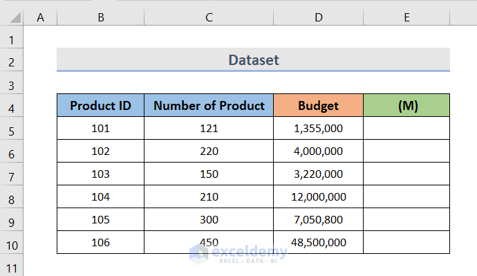
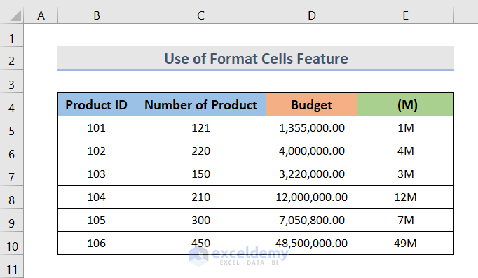
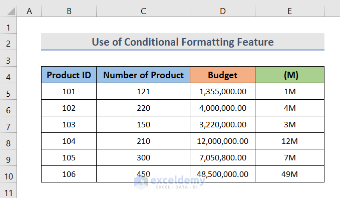
How to Format Number to Millions in Excel (6 Easy Ways)

We are using the dataset which contains some Product ID in column B, the total number of products in column C, and the budget of all the products in column E. We want to format the budget column into millions in column E.

Method 1 – Format Numbers to Millions Using a Simple Formula

STEPS:

Enter the following formula in E5.

=D5/1000000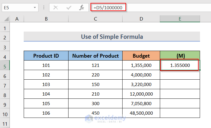

Drag the Fill Handle over the column.

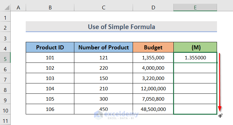
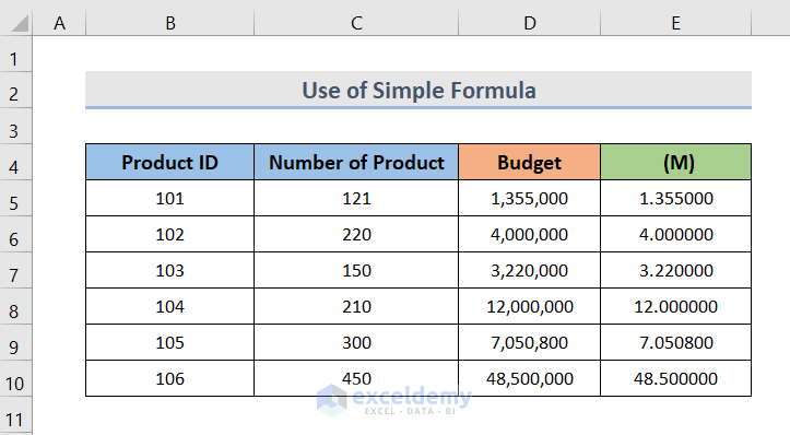
We can see the result in column E.

Method 2 – Insert the ROUND Function to Format Numbers to Millions

STEPS:

Select cell E5.
Insert the following formula and hit Enter.

=ROUND(D5/10^6,1)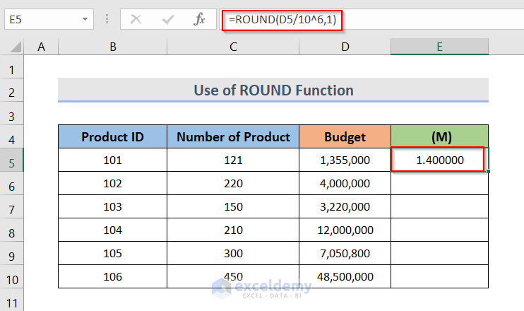

Drag the Fill Handle down.

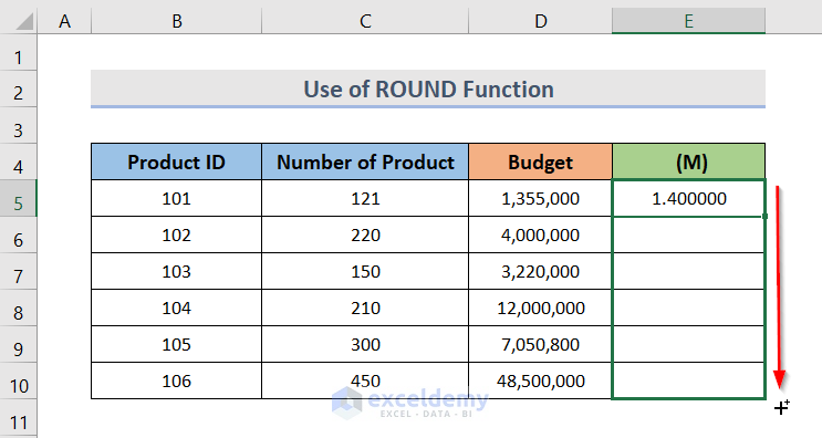
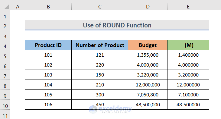
We can see the formatted number.

Method 3 – Use the Paste Special Feature to Format Number to Millions

STEPS:

Insert 1 million anywhere in our workbook. We put it on cell F7.
Copy the cell by pressing Ctrl + C.

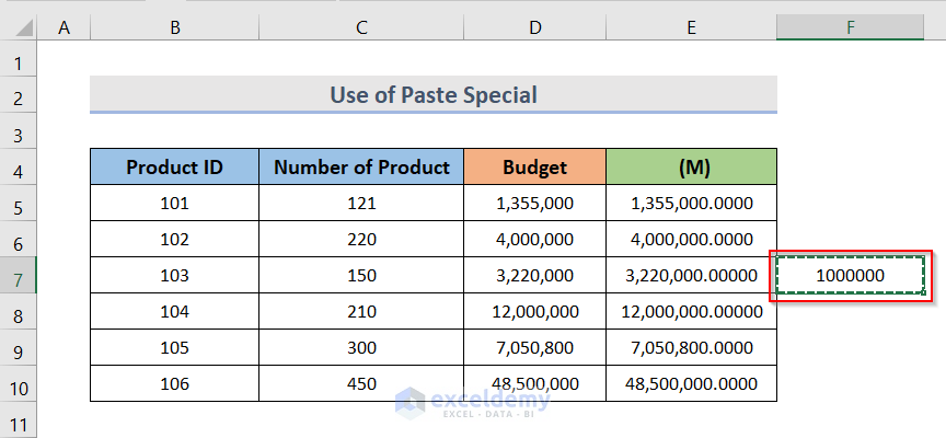
Select the cells where we want to use the paste special feature. We selected cell E5:E10.
Right-click over the selection and click on Paste Special.

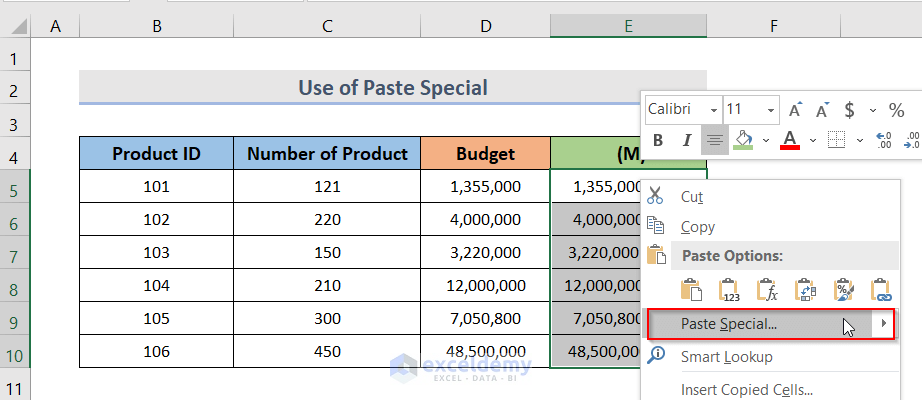
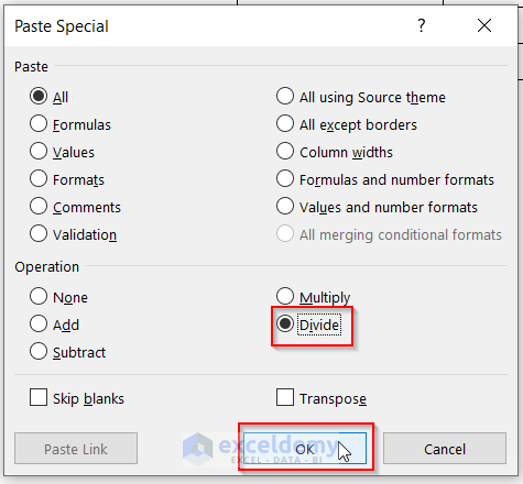
The Paste Special dialog box will appear. Choose the Divide operation.
Click on the OK button.

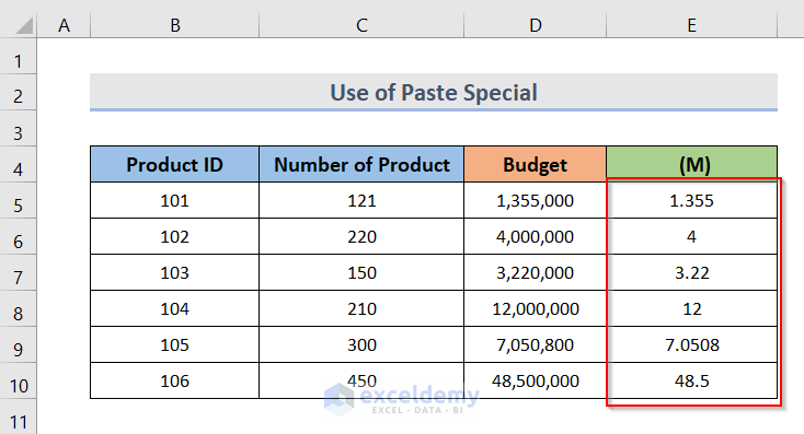
Here’s the result.

Method 4 – Using the TEXT Function for Formatting into Millions

STEPS:

Select cell E5.
Insert the formula below and press Enter.

=TEXT(D5,"#,##0,,")&"M"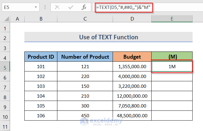

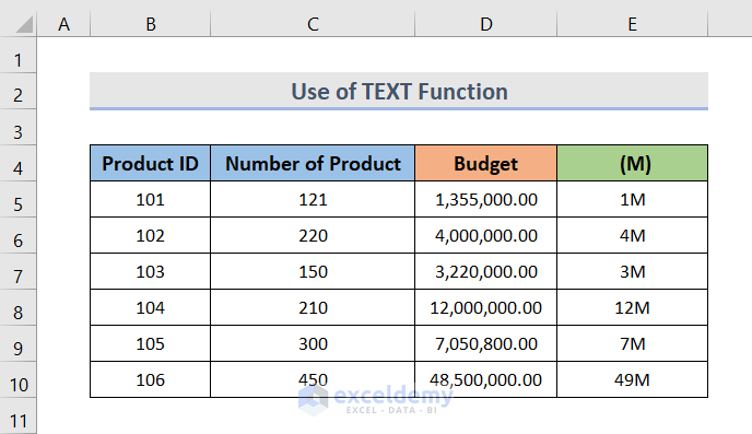
Drag the Fill Handle down.

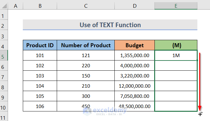
Here’s the result.

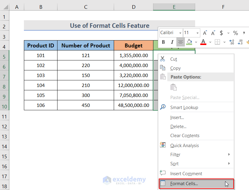
Method 5 – Format Numbers to Millions with the Format Cells Feature

STEPS:

Choose the cells to which you want to apply custom formatting.
Right-click on the selection and choose Format Cells. This will open the Format Cells dialog box.

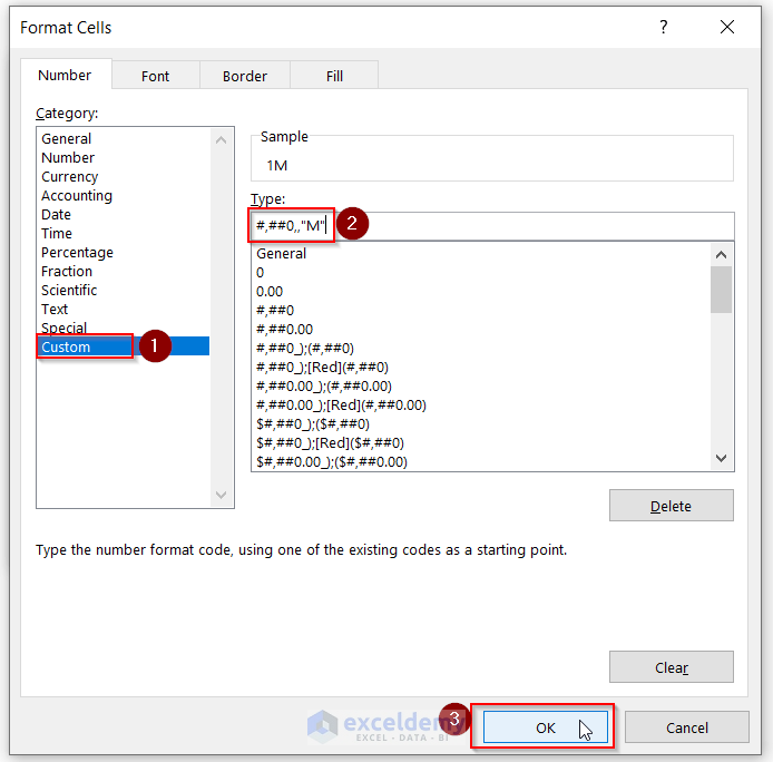
From the Number tab, go to Custom.
In the Type field, type #,##0,,”M”.
Hit OK.

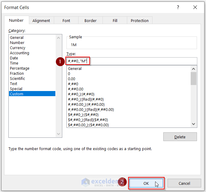
Here’s the result.

Method 6 – Applying Conditional Formatting for the Number Format

STEPS:

Select the range of cells that you want to format.
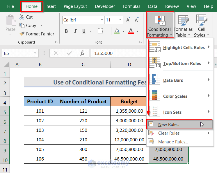
Go to the Home tab in the ribbon.
Click on Conditional Formatting.
From the drop-down menu, select the New Rules option.

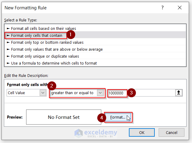
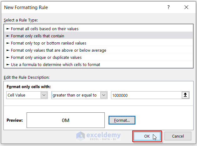
A New Formatting Rule window will appear. Select Format only cells that contain in the Select a Rule Type list.
Select greater than or equal to and type 1000000 for the Format only cells with preferences.
Click on Format.