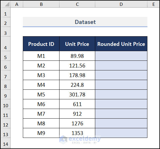
As shown in the following figure, we have the unit price for each Product ID. Let’s round the unit prices to the nearest 100.
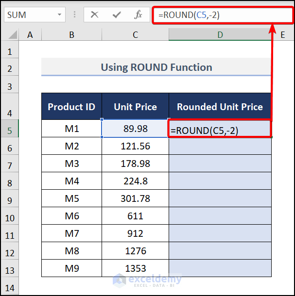
Method 1 – Using the ROUND Function
Steps:
- Go to cell D5 and insert this formula:
C5= The number to be rounded.
-2= The number of digits to which the number should be rounded.
The ROUND(C5, -2) syntax takes C5 as the number to round and “-2” is the number of digits as we want to round the nearest 100.
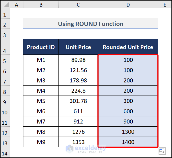
- Press Enter and drag down the Fill Handle tool for other cells.

- You will get your numbers rounded to the nearest 100, just like in the image below.
Read More: Round to Nearest 5 or 9 in Excel
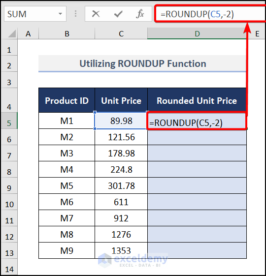
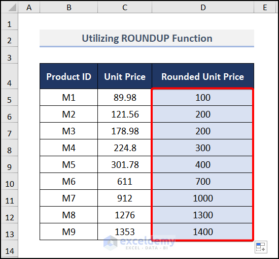
Method 2 – Utilizing the ROUNDUP Function
The ROUNDUP function always rounds a number up.
Steps:
- Move to cell D5 and copy the following formula:
The ROUNDUP(C5, -2) syntax takes C5 as the number to round, and “-2” is the number of digits as we want to round the nearest 100. This function always rounds the function up to the next nearest 100.
- Hir Enter and drag the cell down for other cells in the column.
Read More: How to Round Numbers to the Nearest Multiple of 5 in Excel
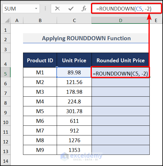
Method 3 – Applying ROUNDDOWN Function
The ROUNDDOWN function always rounds a number down.
Steps:
- Go to cell D5 and enter this formula:
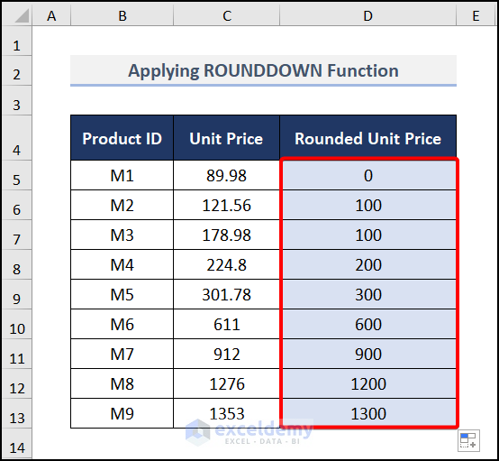
The ROUNDUP(C5, -2) syntax takes C5 as the number to round, and “-2” is the number of digits as we want to round the nearest 100. This function rounds down the number to the nearest 100.
- Press Enter, then use AutoFill for the other cells you need.
Read More: How to Round Numbers in Excel Without Formula
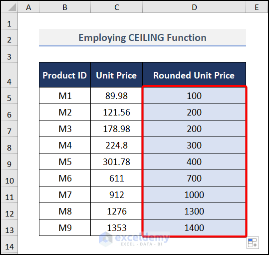
Method 4 – Using the CEILING Function
Steps:
- Insert the following formula in D5.
This CEILING(C5, 100) syntax takes the number to be rounded as C5 and the significance as 100.
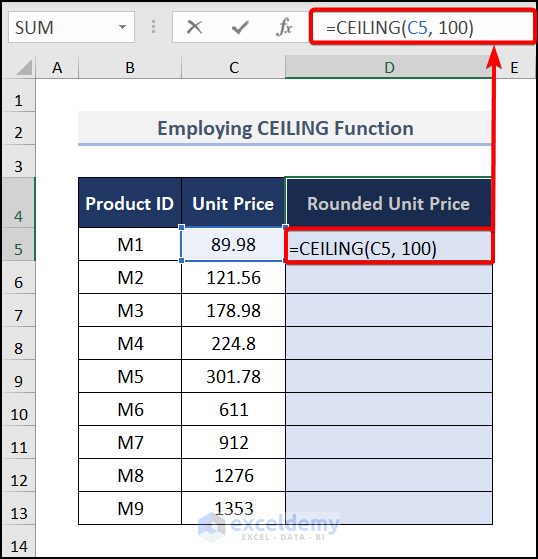
- Hit Enter and AutoFill.
Method 5 – Using the FLOOR Function
Steps:
- Input the following formula in cell D5.
This function takes the number to be rounded as C5 and the significance is 100. It rounds the number down to the below number.
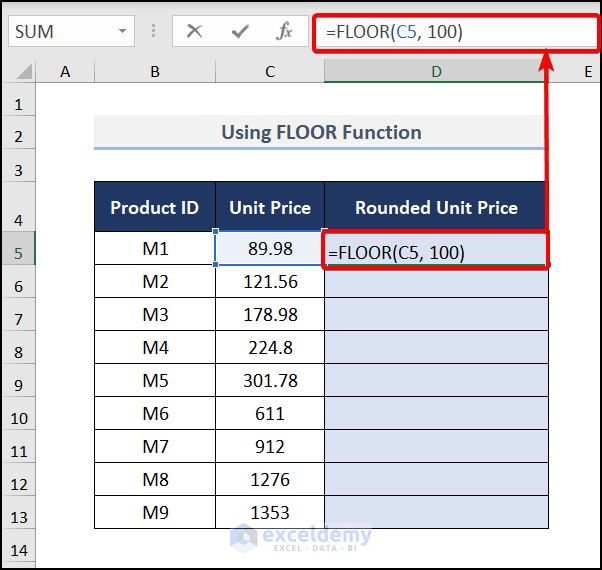
- Hit Enter and use AutoFill.

Read More: Round Down to Nearest 10 in Excel
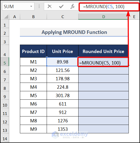
Method 6 – Applying the MROUND Function
Steps:
- Select cell D5 and enter this formula:
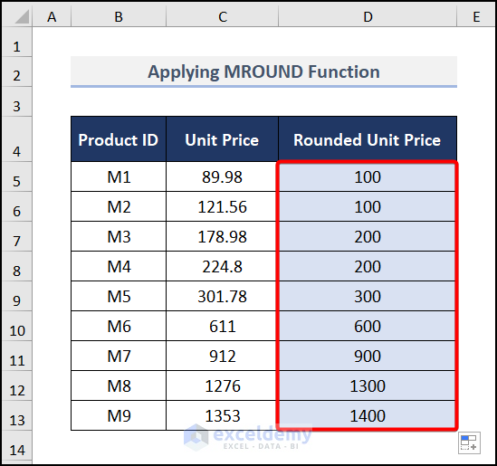
- Press Enter and drag the cell down for other cells.
- You will get the result just like the image below.
Read More: How to Round Numbers to Nearest 10000 in Excel
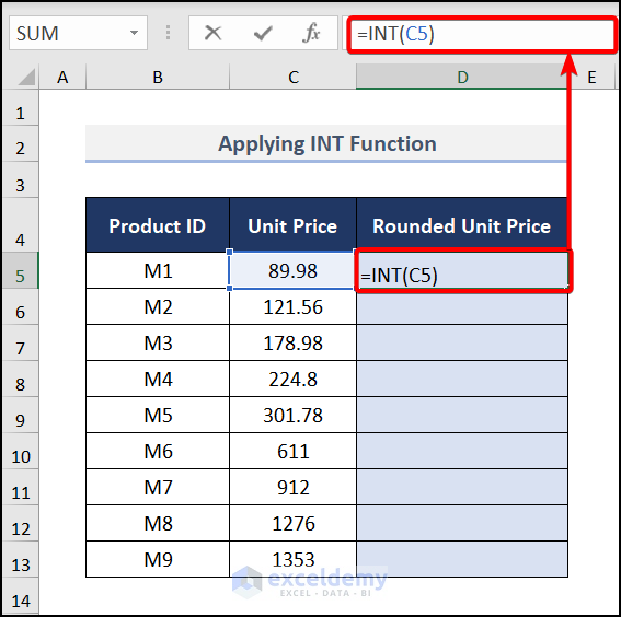
Round to the Nearest Whole Number in Excel
Steps:
- Select cell D5 and enter this formula:
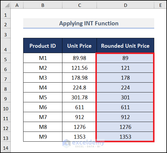
This function rounds the whole number without the fraction.
- Press Enter and apply AutoFill.
Read More: How to Round to Nearest 1000 in Excel
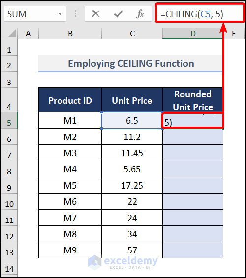
Round to the Nearest 5/1000 in Excel
Steps:
- Use the following formula for D5.
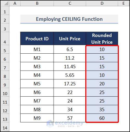
This function rounds the value to the nearest 5 as we insert the significance as 5.
- Hit Enter and AutoFill.
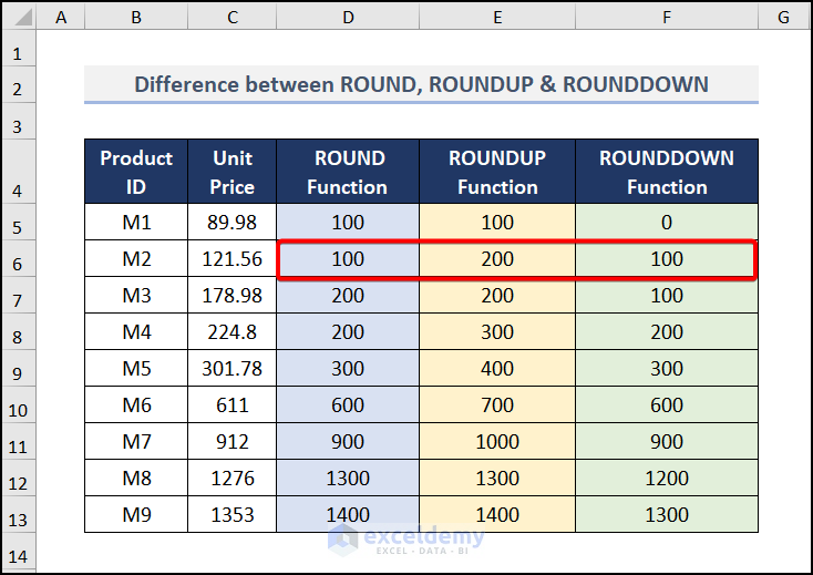
Difference Between ROUND, ROUNDUP, and ROUNDDOWN Functions
See the output of D6, E6, and F6 cells in the following figure. The ROUND function rounds 121.56 to 100, ROUNDUP rounds it up to 200, and ROUNDDOWN rounds it down to 100.
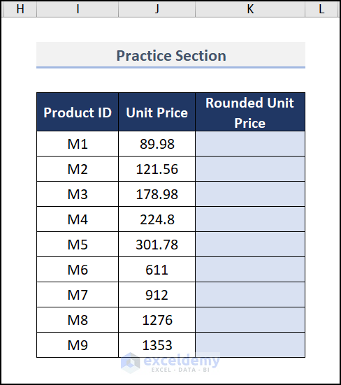
Practice Section
We have provided a practice section on each sheet on the right side so you can apply these methods.
Download the Practice Workbook
Further Readings
- How to Round to Nearest Whole Number in Excel
- How to Round Down to Nearest Whole Number in Excel
- Rounding to Nearest Dollar in Excel
- How to Round to Nearest 10 Cents in Excel
- How to Round Off to Nearest 50 Cents in Excel
<< Go Back to Round to Nearest Whole Number | Rounding in Excel | Number Format | Learn Excel
Get FREE Advanced Excel Exercises with Solutions!
