Method 1 – Using the ROUND Function to Round to Nearest 10000
Steps:
- Enter the formula in cell C5:
=ROUND(B5,-4)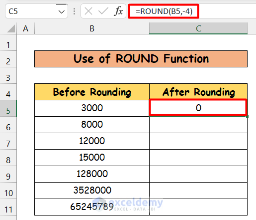
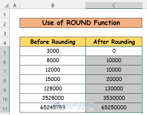
- Use the Fill Handle to copy the formula up to C11.
- We will get our final rounded result.
How Does the Formula Work?
In this formula, firstly, I have initially passed the desired cell number where the number is located, which is B5. We want to round nearest to 10000; that’s why in the second portion, it is -4.
Read More: How to Round to Nearest 100 in Excel
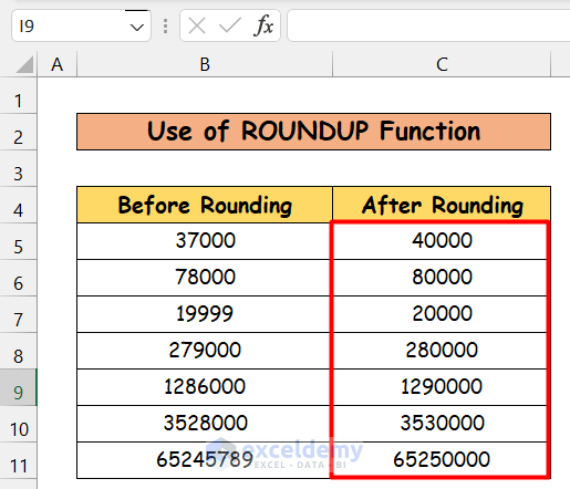
Method 2 – Utilizing the ROUNDUP Function to Round to the Nearest 10000
Steps:
- Enter the formula in cell C5:
=ROUNDUP(B5,-4)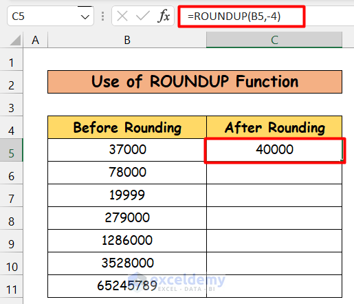
- Using the Fill Handle, copy the formula up to C11.
Read More: How to Round to Nearest 1000 in Excel
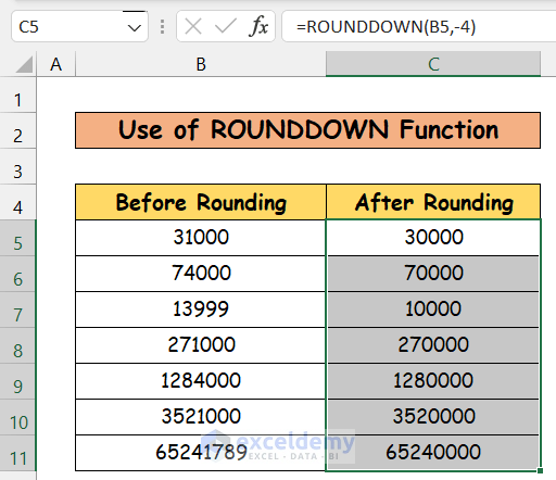
Method 3 – Applying the ROUNDDOWN Function to Round to the Nearest 10000
Steps:
- Enter the formula in cell C5:
=ROUNDDOWN(B5,-4)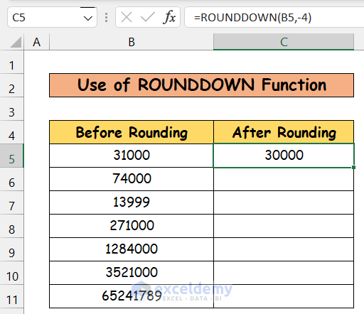
- Copy the formula up to C11.
Read More: How to Round Numbers in Excel Without Formula
Method 4 – Applying CEILING and FLOOR Functions to Round to the Nearest 10000
4.1 Applying CEILING Function
Steps:
- Enter the formula in cell C5:
=CEILING(B5,10000)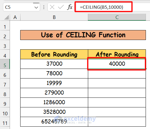
- Copy the formula up to C11.
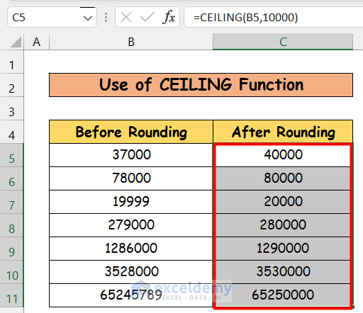
How Does the Formula Work?
In this function firstly, I have passed the cell number (B5) where our number is located. Then as we want to round to the nearest 10000, that’s why I have passed 10000 in the second portion. This will round up to the nearest highest 10000 as much as can.
4.2 Applying FLOOR Function
Steps:
- Enter the formula using the FLOOR function in cell C5:
=FLOOR(B5,10000)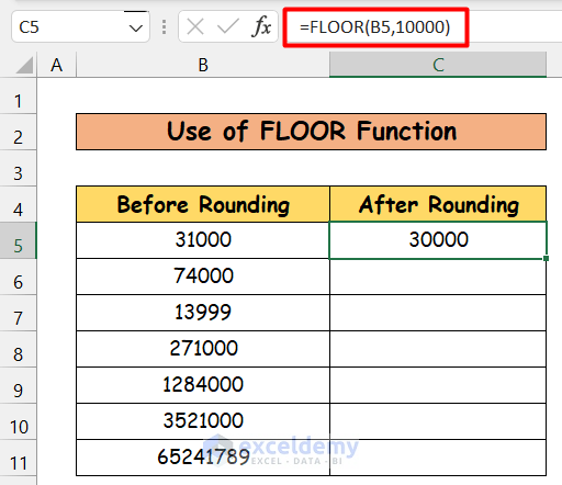
- Copy the formula up to C11.
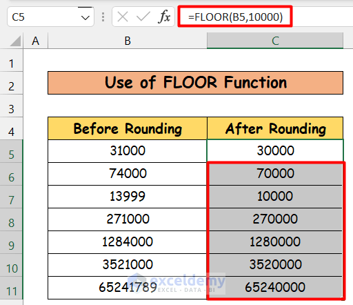
How Does the Formula Work?
In this function, I have first passed the cell number (C5) where our number is located. Then, as we want to round to the nearest 10000, I have passed 10000 in the second portion. This will round up to the nearest lowest 10000 as much as possible.
Method 5 – Using the MROUND Function to Round to the Nearest 10000
Steps:
- Enter the formula in cell C5:
=MROUND(C5,10000)
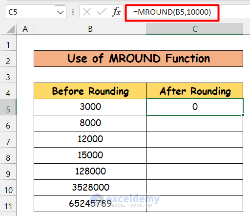
- Copy down the formula up to C11.
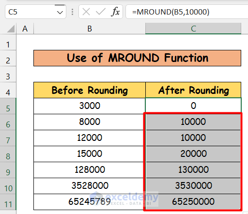
How Does the Formula Work?
As with the previous functions, the number we want to round is in the A5 cell. Then the multiple value is 10000 as we want to find out the round to the nearest 10000.
Read More: How to Round Numbers to the Nearest Multiple of 5 in Excel
Download the Practice Workbook
Download this workbook to practice.
Further Readings
- How to Round to Nearest Whole Number in Excel
- How to Round Down to Nearest Whole Number in Excel
- Round to Nearest 5 or 9 in Excel
- Round Down to Nearest 10 in Excel
- Rounding to Nearest Dollar in Excel
- How to Round to Nearest 10 Cents in Excel
- How to Round Off to Nearest 50 Cents in Excel
<< Go Back to Round to Nearest Whole Number | Rounding in Excel | Number Format | Learn Excel
Get FREE Advanced Excel Exercises with Solutions!
