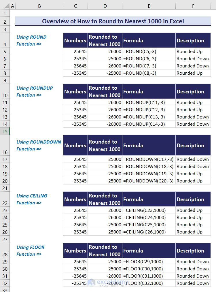
Here’s an overview of the different ways you can round numbers to the nearest 1,000. Let’s dig into each option.
Method 1 – Using Excel ROUND Function to Round Numbers to Nearest 1000
The ROUND function round numbers to the nearest 1,000 based on general math rules. If the hundreds place digit of a number is less than 5, then the hundreds place is replaced by 0. If the hundreds place digit of a number is greater than or equal to 5, then the hundreds place is replaced by 0 and the thousands place is increased by 1.
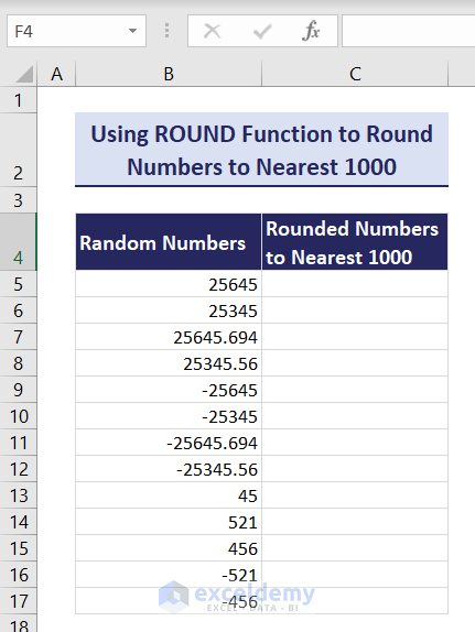
Let’s use a dataset with some random numbers. There are both positive and negative integers and decimal numbers in the dataset. I want to round the numbers to the nearest 1,000.
Steps:
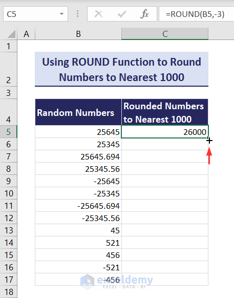
- Copy this formula in cell C5:
=ROUND(B5,-3)
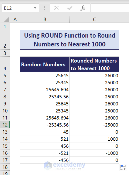
- Hit Enter button and you will find the following output. Hover your mouse over the bottom right corner of cell C5 to find the Fill Handle icon (Plus).
- Double-click on the Fill Handle icon to round all the numbers to the nearest 1,000 across cells C5:C17.
Read More: How to Round Numbers to Nearest 10000 in Excel
Method 2 – Using Excel ROUNDUP Function to Round Numbers to Nearest 1000
Excel ROUNDUP function rounds up positive numbers and rounds down negative numbers.
Steps:
- Copy this formula in cell C5:
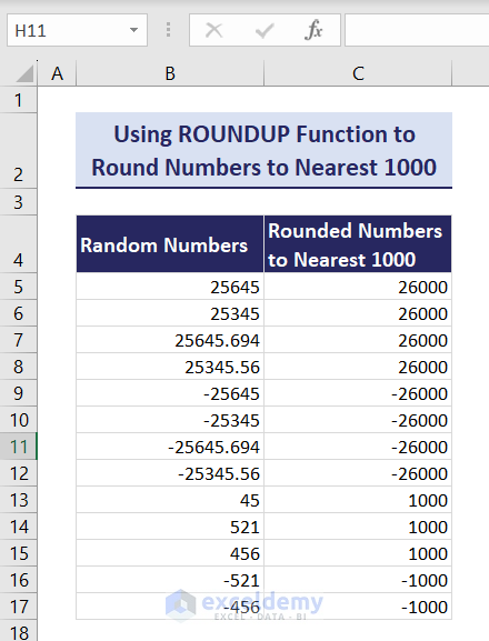
=ROUNDUP(B5,-3)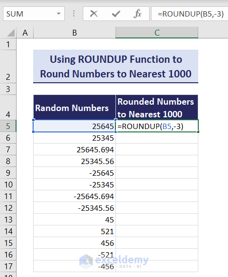
- Press Enter.
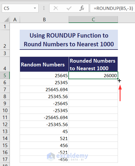
- Double-click on the Fill Handle icon (bottom right corner of the cell C5) to round all the numbers to the nearest 1,000 across the cells C5:C17.
Read More: How to Round to Nearest 100 in Excel
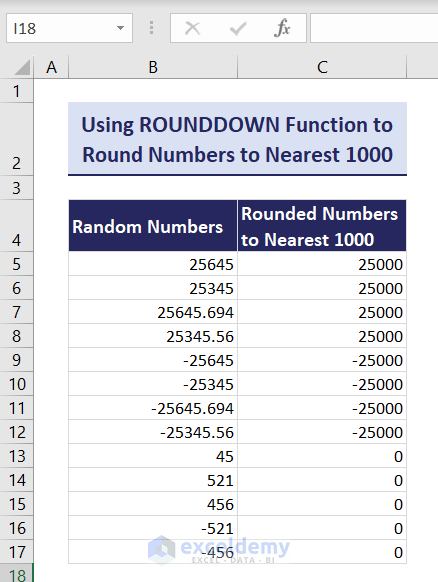
Method 3 – Using Excel ROUNDDOWN Function to Round Numbers to Nearest 1000
Excel’s ROUNDDOWN function rounds down positive numbers and rounds up negative numbers.
Steps:
- Insert this formula in cell C5:
=ROUNDDOWN(B5,-3)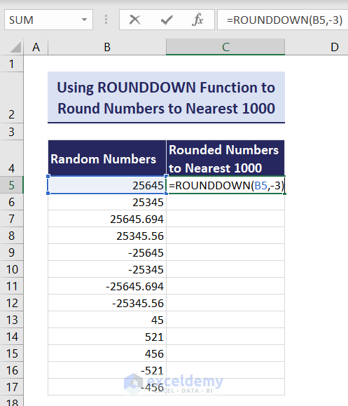
- Hit Enter.
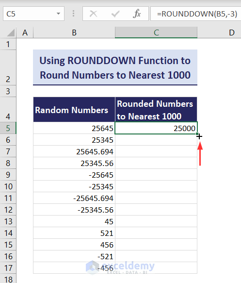
- Double-click on the Fill Handle icon (bottom-right corner of C5) to round all the numbers to the nearest 1,000 across cells C5:C17.
Read More: Round Down to Nearest 10 in Excel
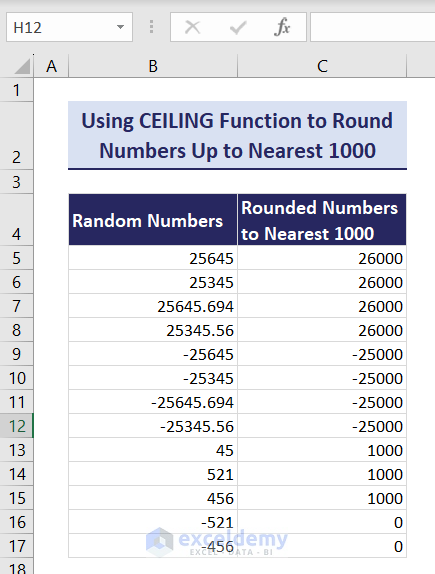
Method 4 – Using Excel CEILING Function to Round Numbers to Nearest 1000
Case 1 – Rounding Numbers Up to Nearest 1000 Using CEILING Function
Steps:
- Copy this formula in cell C5:
=CEILING(B5,1000)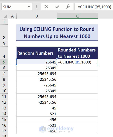
- Hit Enter.
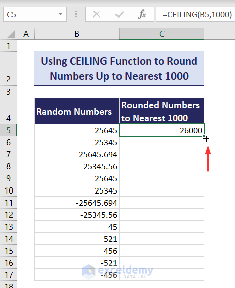
- Double-click on the Fill Handle icon (bottom-right corner of C5) to round all the numbers up to the nearest 1,000 across the range C5:C17.
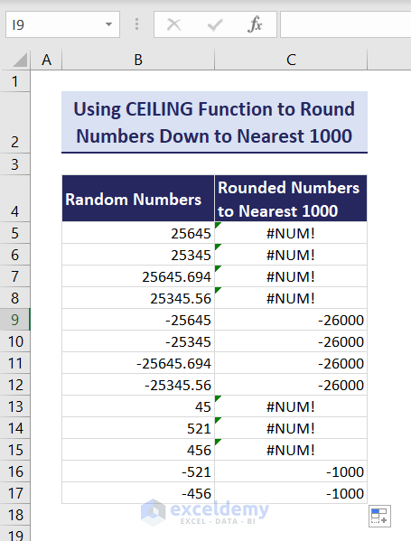
Case 2 – Rounding Numbers Down to Nearest 1000 Using CEILING Function
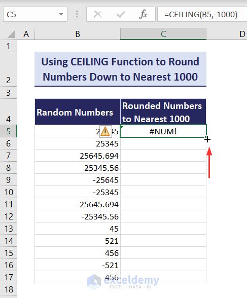
Excel’s CEILING function rounds down only negative numbers when the significance argument is negative. When the number is positive and the significance argument is negative, Excel CEILING function returns a #NUM! error.
Steps:
- Copy this formula in cell C5:
=CEILING(B5,-1000)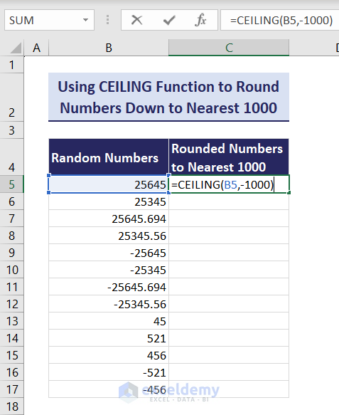
- Hit Enter.
- Double-click on the Fill Handle icon (bottom-right corner of C5) to round only the negative numbers down to the nearest 1,000 across cells C5:C17.
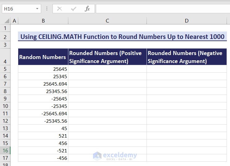
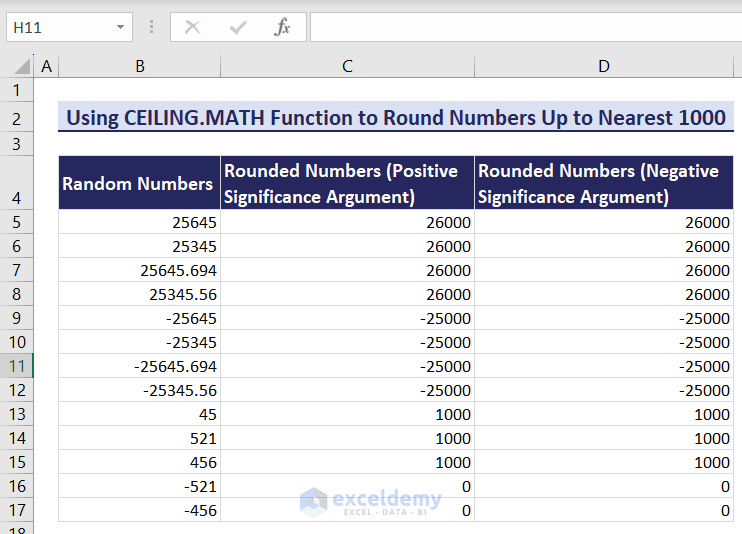
Method 5 – Using Excel CEILING.MATH Function to Round Numbers Up to Nearest 1000
We’ll use the following dataset and will use the CEILING.MATH function with positive significance argument and negative significance argument in separate columns to round the numbers up to the nearest 1,000.
Steps:
- Copy this formula in cell C5:
=CEILING.MATH(B5,1000)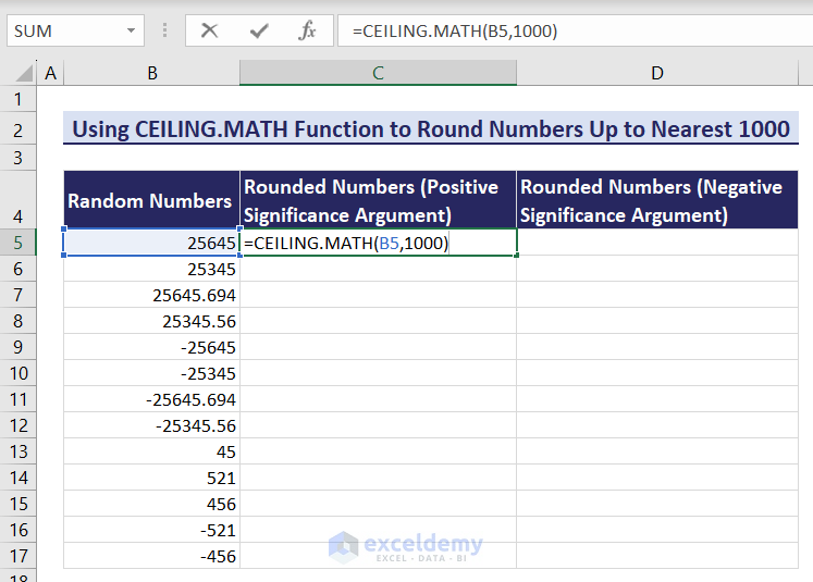
- Hit Enter.

- Double-click on the Fill Handle icon (bottom-right corner of cell C5) to round all the numbers up to the nearest 1,000 across cells C5:C17.
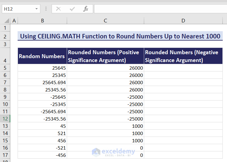
- Copy this formula in cell D5:
=CEILING.MATH(B5,-1000)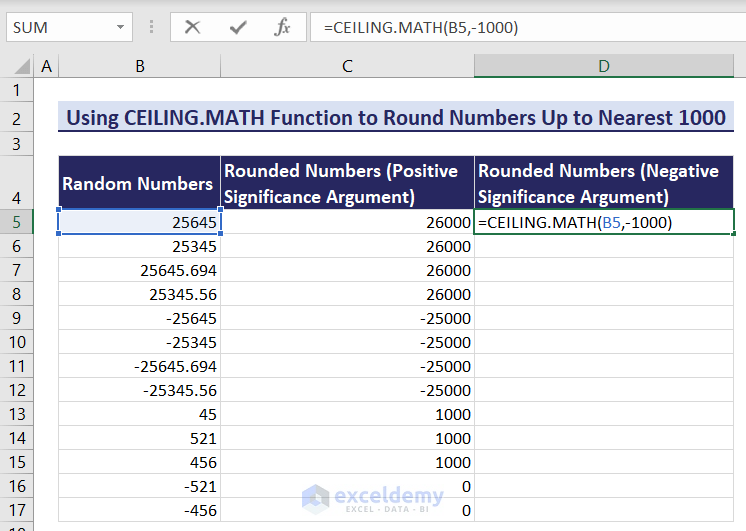
- Hit Enter.
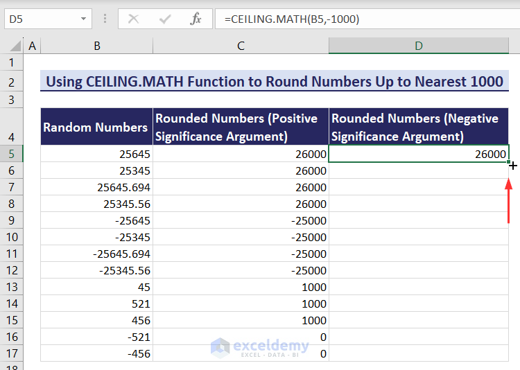
- Double-click on the Fill Handle icon.
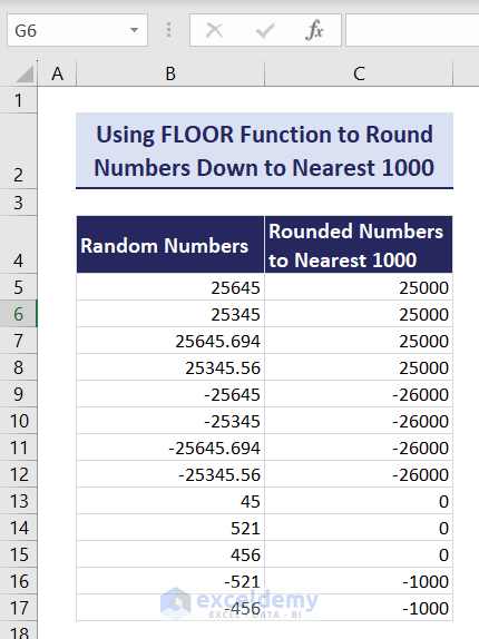
Method 6 – Using Excel FLOOR Function to Round Numbers to Nearest 1000
Case 1 – Rounding Numbers Down to Nearest 1000 Using FLOOR Function
The FLOOR function rounds down both the positive and negative numbers when the significance argument is positive.
Steps:
- Copy this formula in cell C5:
=FLOOR(B5,1000)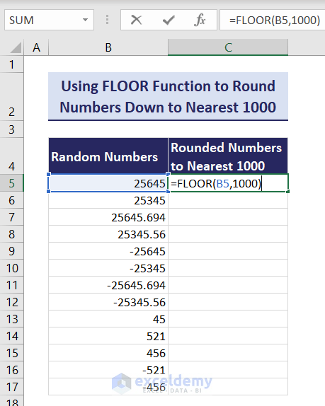
- Hit Enter.
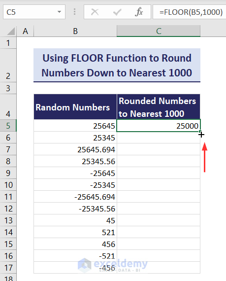
- Double-click on the Fill Handle icon (bottom-right corner of cell C5).
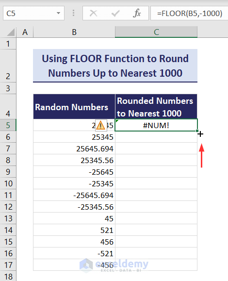
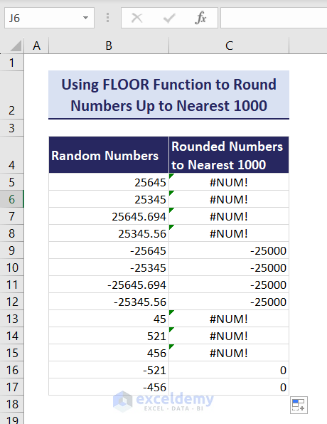
Case 2 – Rounding Numbers Up to Nearest 1000 Using FLOOR Function
Excel FLOOR function rounds up only negative numbers when the significance argument is negative. When the number is positive and the significance argument is negative, Excel FLOOR function returns a #NUM! error.
Steps:
- Copy the following formula in cell C5:
=FLOOR(B5,-1000)
- Press Enter.
- Double-click on the Fill Handle icon (bottom-right corner of cell C5).
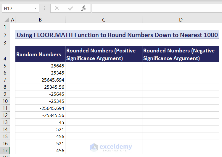
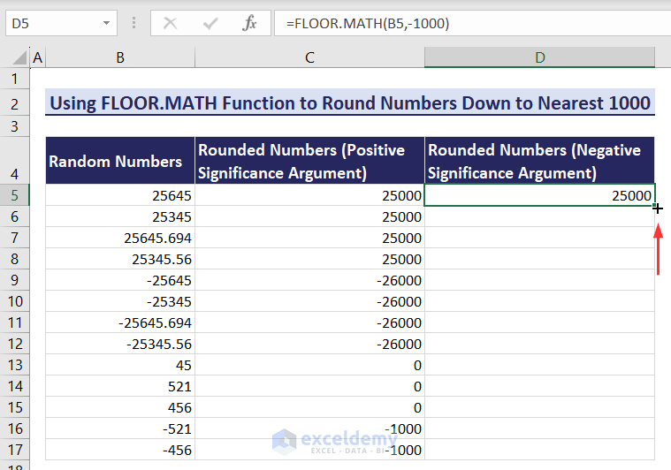
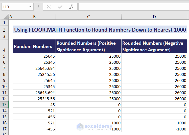
Method 7 – Using Excel FLOOR.MATH Function to Round Numbers Down to Nearest 1000
The FLOOR.MATH function rounds down both the positive and negative numbers. We’ll use the following dataset and will use the FLOOR.MATH function with positive significance argument and negative significance argument in separate columns to round the numbers down to the nearest 1000.
Steps:
- Copy the following formula in cell C5:
=FLOOR.MATH(B5,1000)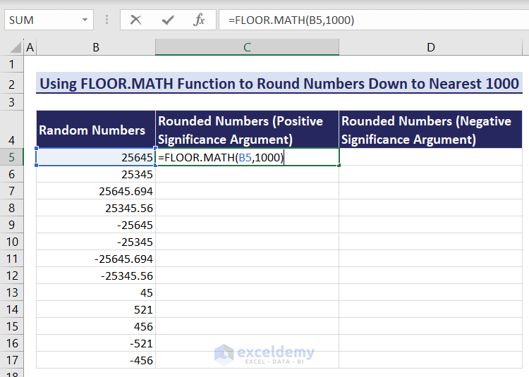
- Press Enter.
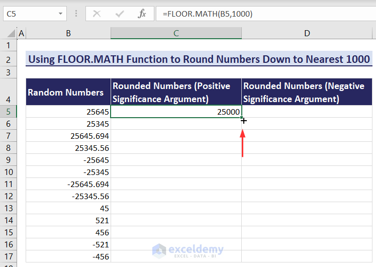
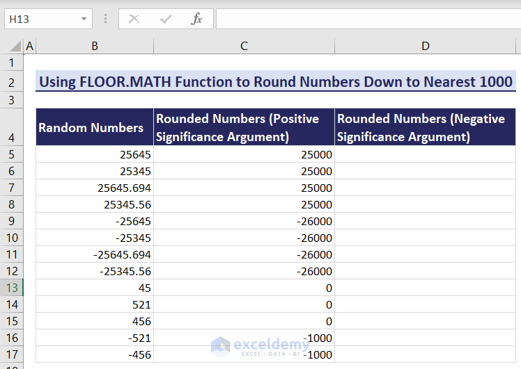
- Double-click on the Fill Handle icon (bottom-right corner of C5) to copy the formula throughout the column.
- Input this formula in cell D5:
=FLOOR.MATH(B5,-1000)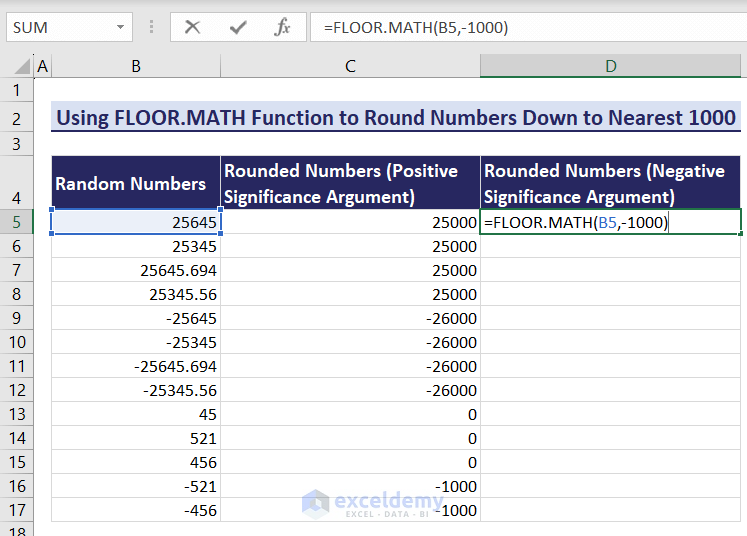
- Hit Enter.
- Double-click on the Fill Handle icon for D5.
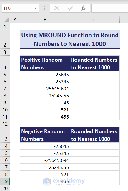
Method 8 – Using Excel MROUND Function
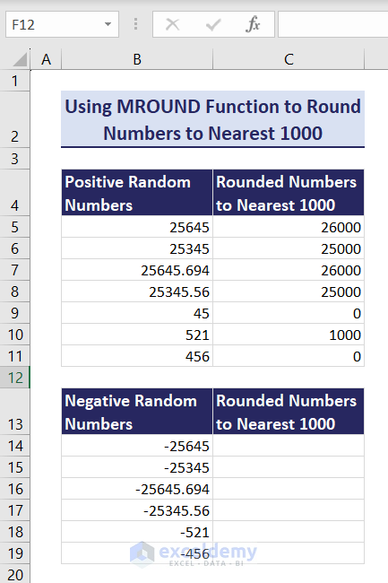
The MROUND function rounds numbers based on general math rules like Excel ROUND function, but both the number and multiple arguments of the MROUND function should have the same sign. We’ll use the following dataset and use the MROUND function for the positive and negative numbers separately to round them to the nearest 1000.
Steps:
- Insert this formula in C5:
=MROUND(B5,1000)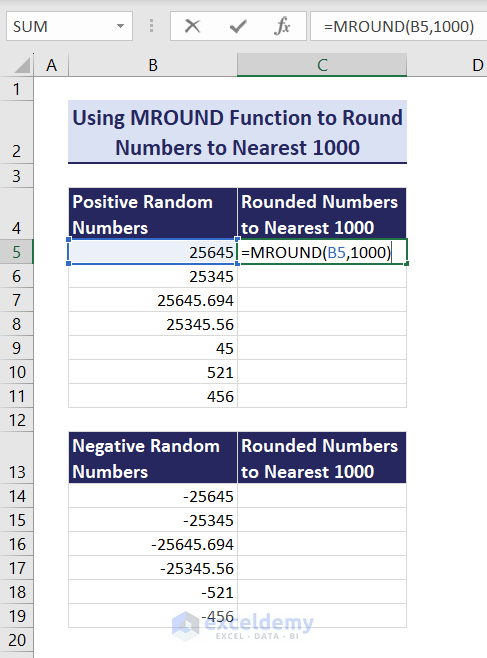
- Hit Enter.
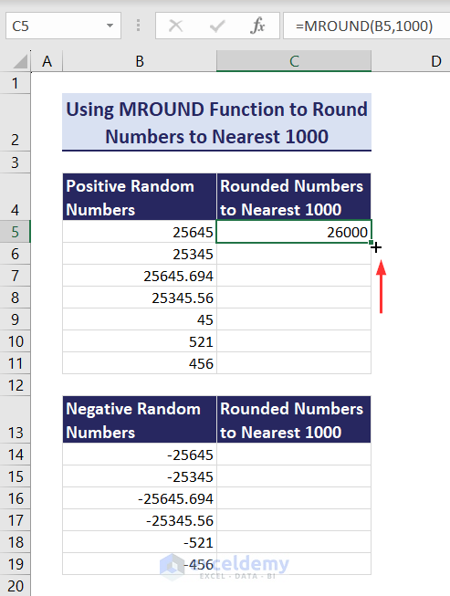
- Double-click on the Fill Handle icon (bottom-right corner of C5).
- Input this formula in C14:
=MROUND(B5,-1000)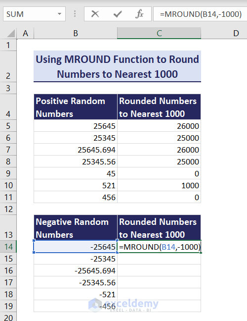
- Press Enter and hover over the bottom-right corner of the cell.
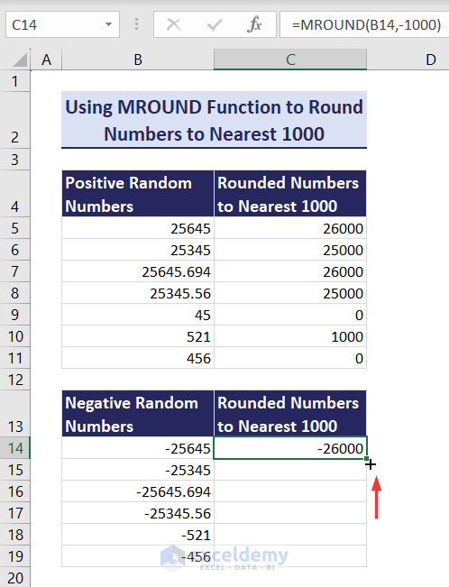
- Double-click on the Fill Handle icon.

Method 9 – Combining Excel SIGN, ABS and MROUND Functions
Steps:
- Copy this formula into cell C5:
=SIGN(B5)*MROUND(ABS(B5),ABS(1000))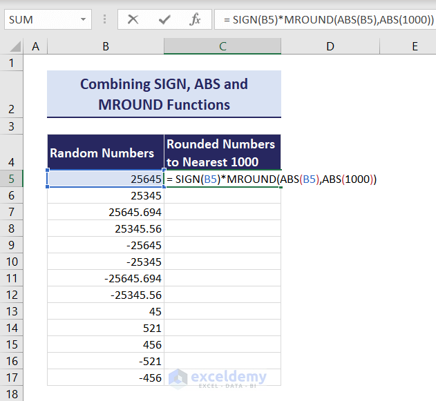
- Hit Enter and hover over the bottom right corner of cell C5 to find the Fill Handle icon.
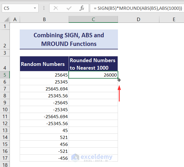
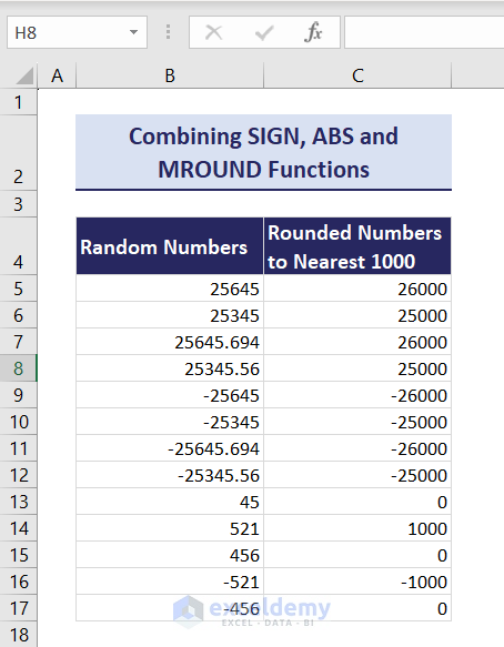
- Double-click on the Fill Handle icon to copy the formula to the other cells in the column.
Formula Breakdown:
Let’s explain how this formula works:
=SIGN(B5)*MROUND(ABS(B5),ABS(1000))
=SIGN(B5)*MROUND(25645,1000) // ABS(B5) returns 25645 and ABS(1000) returns 1000 as the absolute value.
=SIGN(B5)*MROUND(25645,1000)
=SIGN(B5)*26000 // MROUND(25645,1000) returns 26000 because this function rounds the value 25645 to the nearest 1000.
=1*26000 // SIGN(B5) returns 1 because the number in cell B5 is positive.
=26000 // Because the multiplication result is 26000.
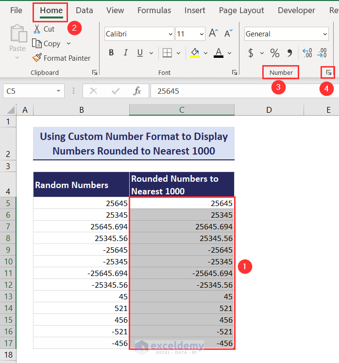
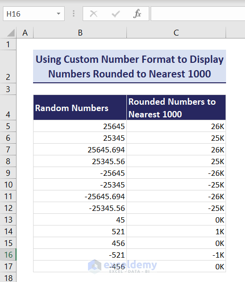
Method 11 – Using Custom Number Format to Display Numbers Rounded to Nearest 1000
Let’s copy the original values and paste them into another column, then use the Custom Number Format option to display the numbers rounded to the nearest 1,000.
Steps:
- Select cells B5:B17.
- Press Ctrl + C to copy.
- Select cell C5.
- Press Ctrl + V to paste.
- Select cells C5:C17.
- Go to Home tab and the Number group of commands.
- Select the small arrow at the bottom-right of the group.
- The Format Cells dialog box will open.
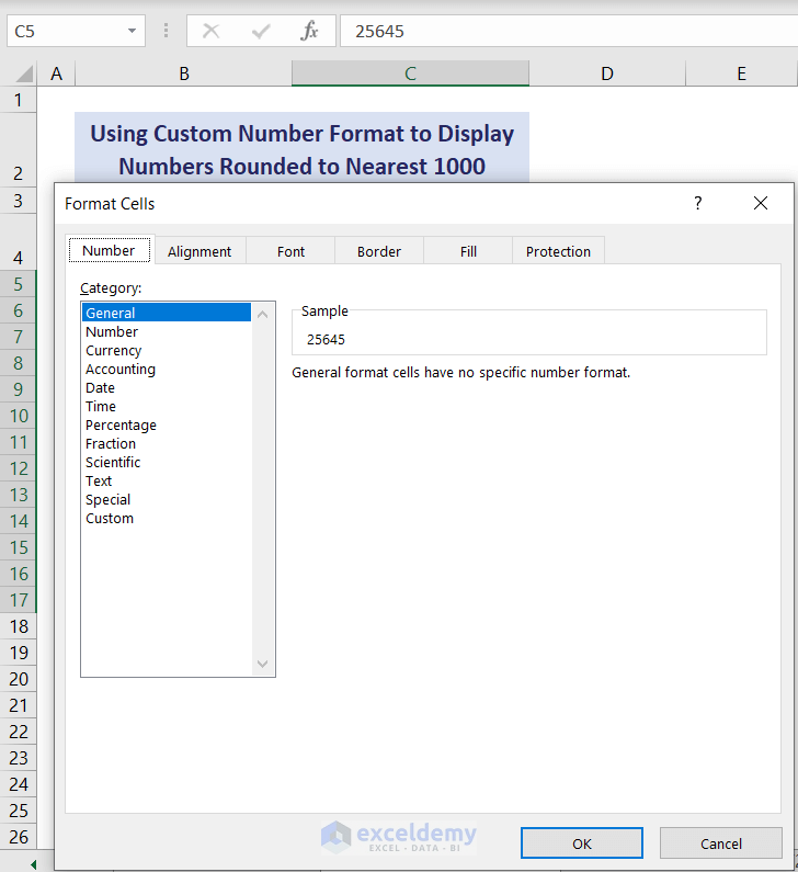
- Go to Number tab.
- Choose Custom from Category.
- Put #0,”000″ in the “Type:” box.
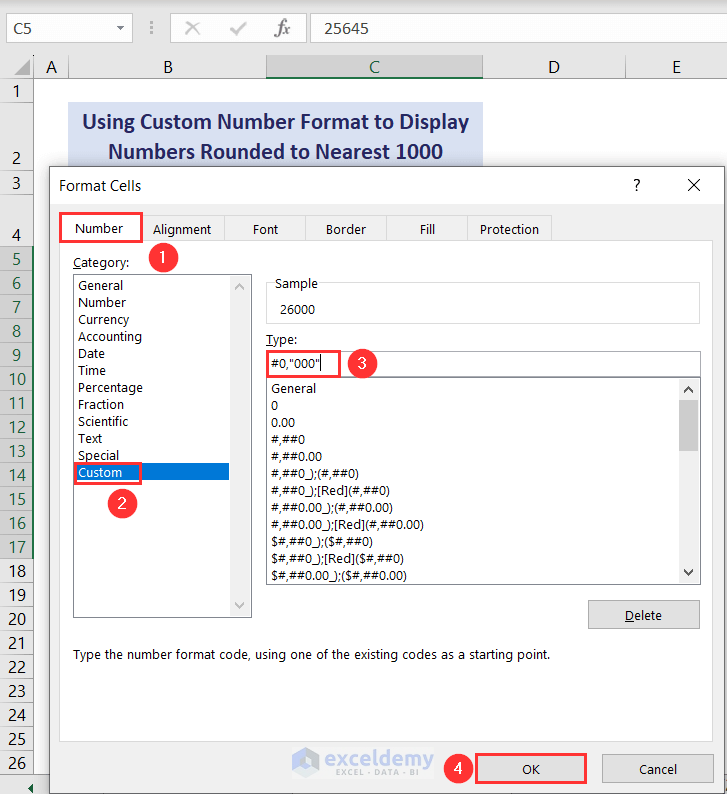
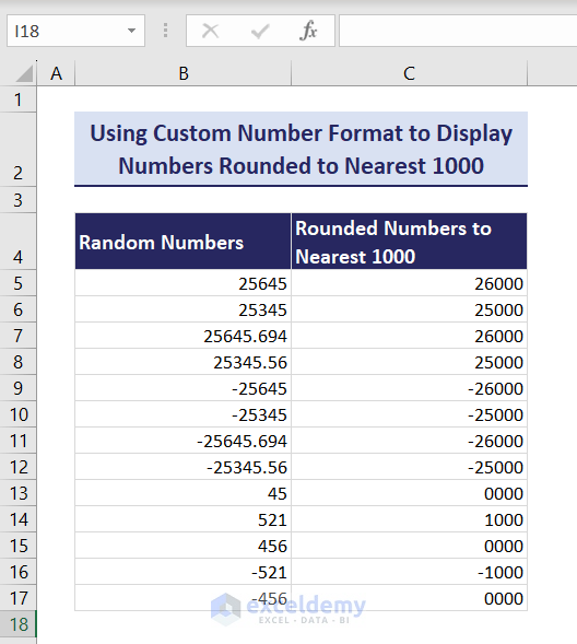
- Click OK and you’ll get the following output.
You can also put #0,”K” in the Type: box.
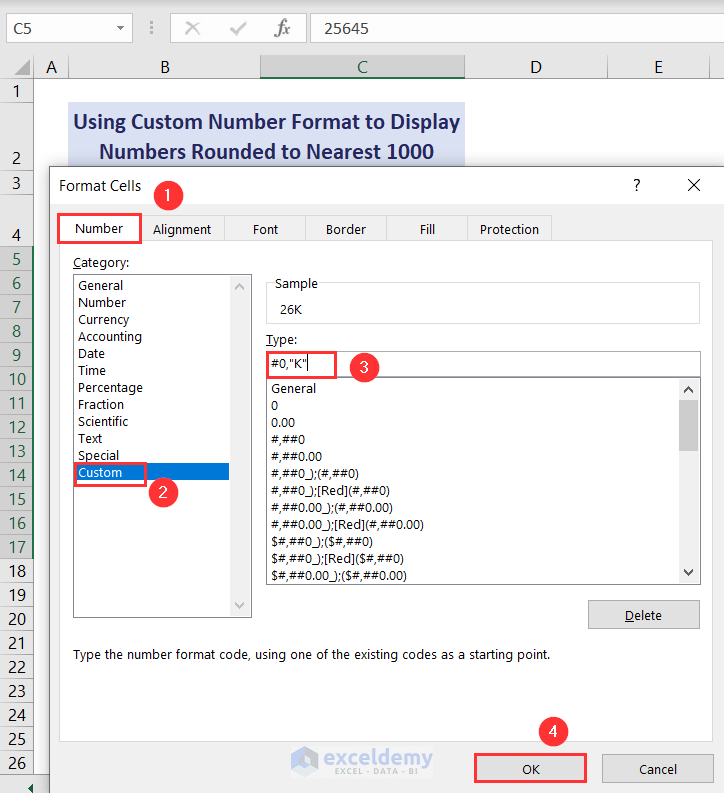
Click OK and you’ll get the following output.
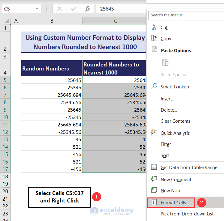
You can also open the Format Cells dialog box in these three ways:
- Select cells C5:C17 and right-click then select the Format Cells option.
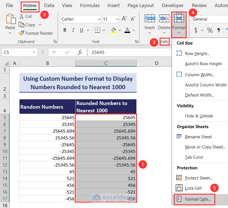
- Select cells C5:C17, go to Home tab, click on the Format drop-down, and choose Format Cells option.
 Select cells C5:C17 and press the keyboard shortcut Ctrl + 1.
Method 11 – Rounding Numbers to Nearest 1000 Using Power Query in Excel
Case 1: Using Number.Round Function
The Number.Round function in Excel Power Query rounds numbers based on general math rules like the Excel ROUND function.
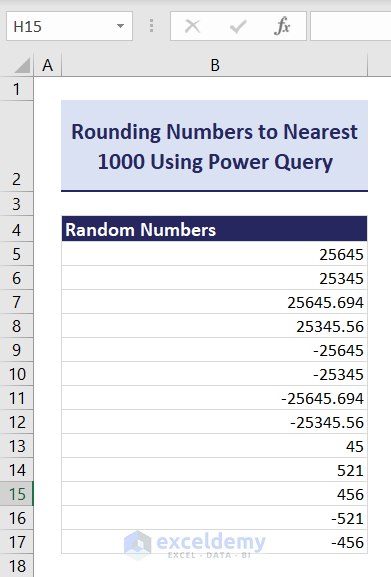
Here’s a dataset with some random numbers with both positive and negative integers and decimal numbers. We want to round the numbers to the nearest 1,000.
Follow these steps:
- Select the whole dataset.
- Go to Data tab and the Get & Transform Data group of commands, then select the From Table/Range option.
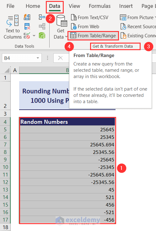
- Click on the From Table/Range option and the Create Table dialog box will open.
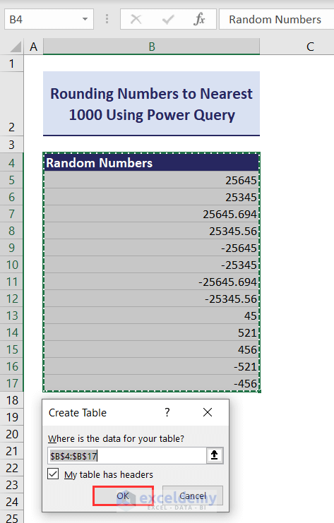
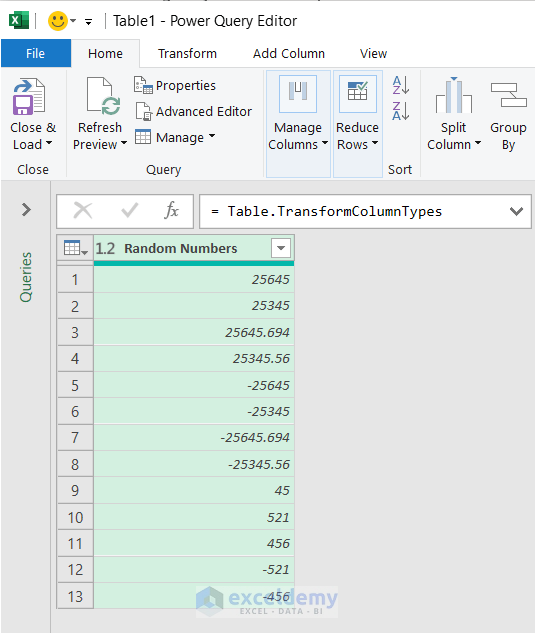
- Click OK and the dataset will import into the Power Query Editor.

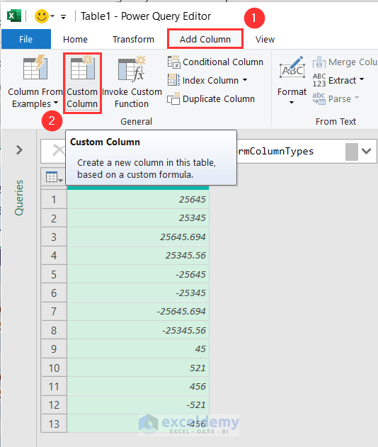
- In the Power Query Editor, go to the Add Column tab and choose the Custom Column option.

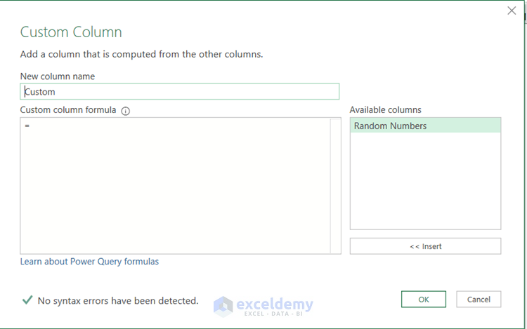
- Click on the Custom Column option and the Custom Column window will open.

- Make a new column name (Rounded Numbers to Nearest 1000) in the New column name box
- Copy this formula in the Custom column formula box:
=Number.Round([Random Numbers], -3)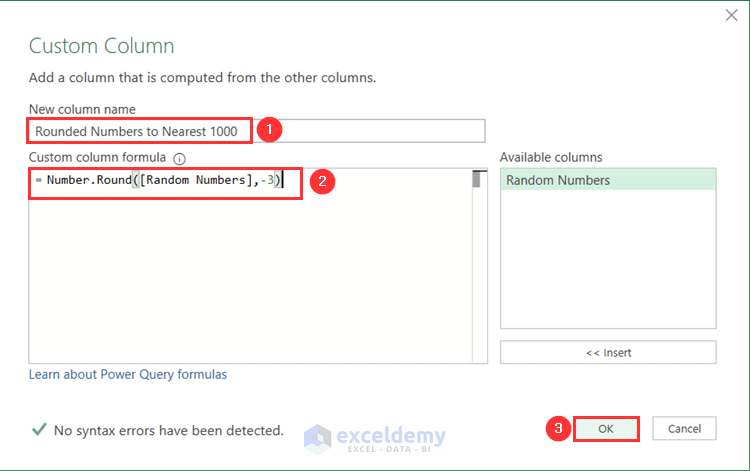
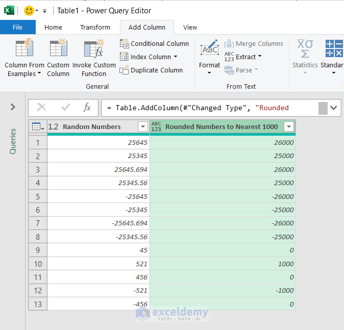
- Click OK to round all the numbers to the nearest 1,000.
- Go to Home tab and click on the Close & Load drop-down. You’ll get the Close & Load To option.
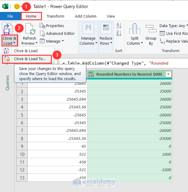
- Click on the Close & Load To option and the Import Data dialog box will appear.
- Select the Table radio button.
- Select the New worksheet radio button as the location.
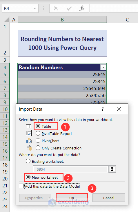
- Click OK and the dataset will export back to the worksheet with the results.
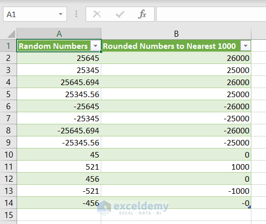
Case 2 – Using Number.RoundUp Function
The Number.RoundUp function rounds up both positive and negative numbers.
Follow these steps:
- Follow the previous case to upload the dataset in Excel Power Query.

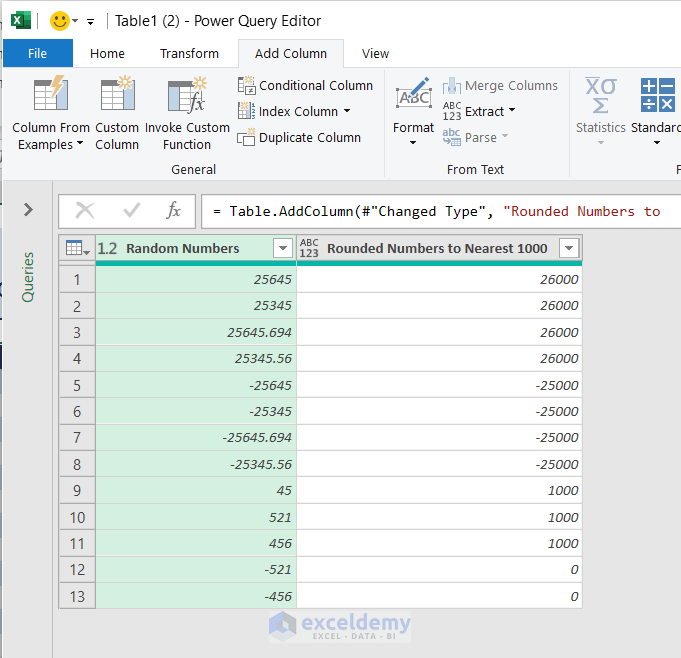
- In the Power Query Editor, go to the Add Column tab and select the Custom Column option.

- The Custom Column window will open.

- Put this formula in Custom column formula box:
=Number.RoundUp([Random Numbers], -3)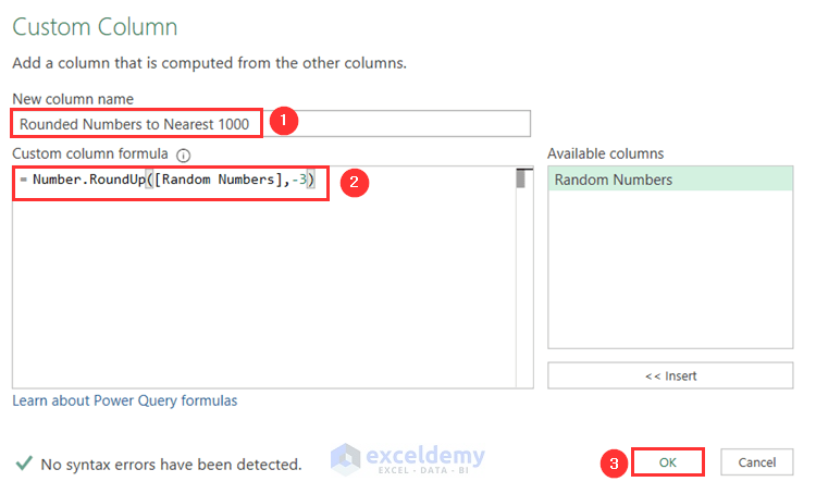
- Click OK to round all the numbers up to the nearest 1,000.
 Follow the rest of the instructions in the previous case.
Case 3 – Using Number.RoundDown Function
The Number.RoundDown function rounds down both positive and negative numbers.
Follow these steps:
Importing the dataset in Power Query
- Follow steps from Case 1 to upload the dataset in Excel Power Query.
- In the Power Query Editor, go to the Add Column tab and select the Custom Column option.
- The Custom Column window will open.
- Input a new column name in the New column name box
- Put this formula in Custom column formula box:
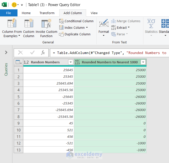
=Number.RoundDown([Random Numbers], -3)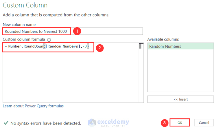
- Click OK to round all the numbers down to the nearest 1000.
- You can load this dataset with the result again in the worksheet by following steps from Case 1.
Download Workbook
Related Articles
- How to Round to Nearest Whole Number in Excel
- How to Round Down to Nearest Whole Number in Excel
- Round to Nearest 5 or 9 in Excel
- How to Round Numbers to the Nearest Multiple of 5 in Excel
- Rounding to Nearest Dollar in Excel
- How to Round to Nearest 10 Cents in Excel
- How to Round Off to Nearest 50 Cents in Excel
<< Go Back to Round to Nearest Whole Number | Rounding in Excel | Number Format | Learn Excel
Get FREE Advanced Excel Exercises with Solutions!

is there a video on this, if not, pl make a video so that it can be understood very easily.
it is difficult to read and understand. If the same is explained in a video it can be understood very easily.
Hello N R RAVINDREA!
Thank you for your suggestion. We are taking this into concern. And, You can share your Excel-related problems in an email at [email protected]
Thank You!
How can we roundUp to first decimal in cell formatting itself (without using formulae)?
E.g
1. If I write 44.41 it show 44.5
2. If I write 44.45 it shows 44.5
3. If I write 44.49 it show 44.5
Hello ISH SHARMA!
You can increase and decrease decimal digits from the format options. But Through this, it will round to the nearest decimal. Suppose, when you round the value 44.41, it will be rounded to 44.4, not 44.5 and for the value 44.45, it will become 44.5.
To use this method,
>> Select the cell.
>> Go to the Home tab in the top ribbon.
>> Here, in the Number menu, click on the “Increase Decimal” icon to increase the decimal digits after the point, and click on the “Decrease Decimal” to decrease the decimal digits.
I hope, your problem will be solved in this way. You can share more problems in an email at [email protected]