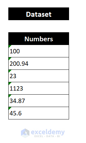
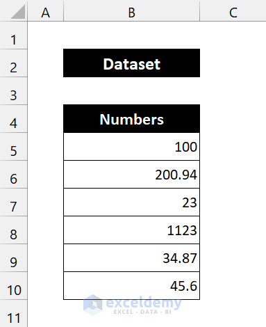
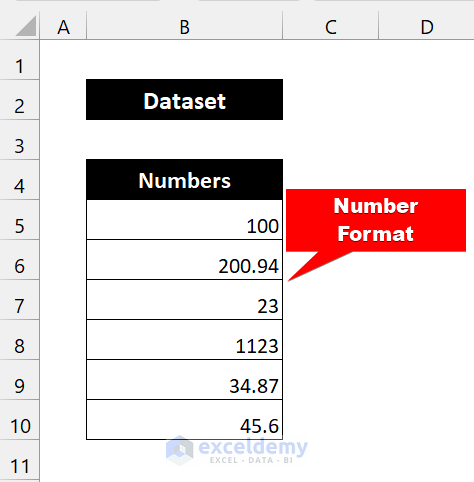
Below is a dataset with some formatted numbers.
Method 1 – Using the Number Format Command
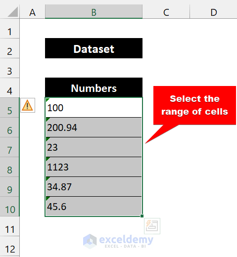
Steps:
- Select the range of cells B5:B10.
- From the Home tab, select Number format from Number.
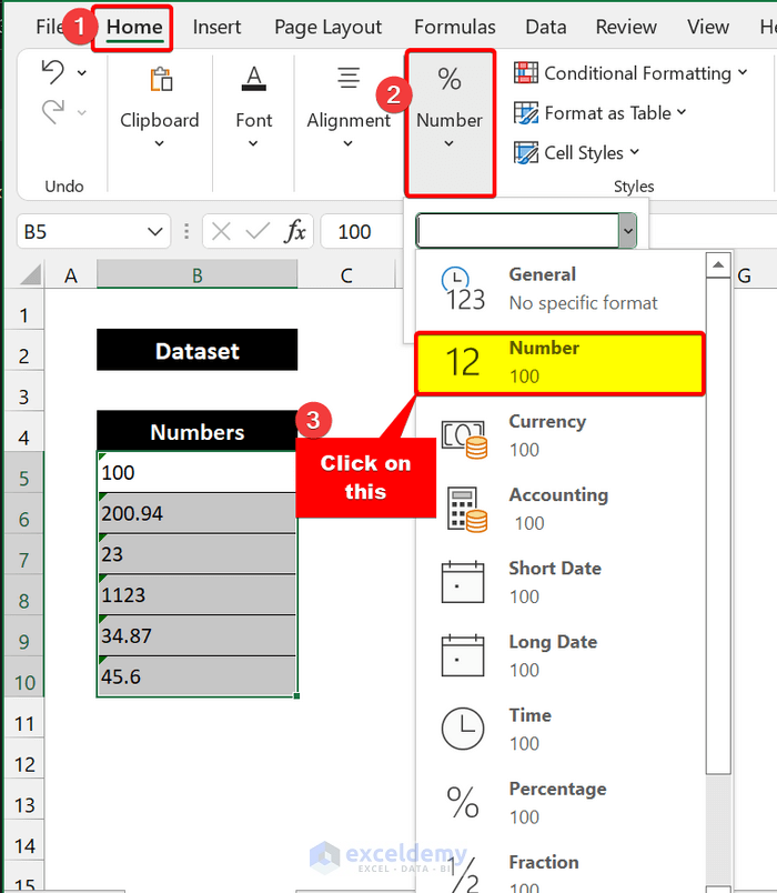
- This will convert your data to a number format.
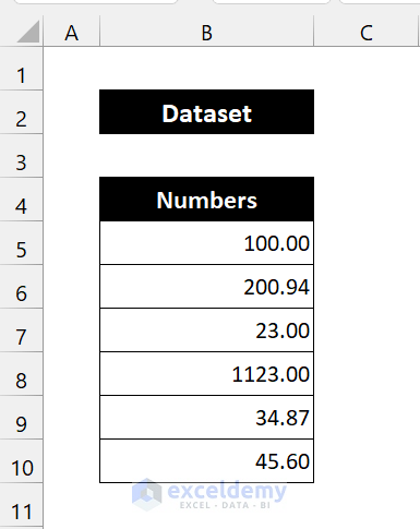
- If you click General format instead of Number, it will look like this:
Both are in the number formats.
- Choose your option according to your problem.
Read More: Excel Number Format Not Working (2 Reasons with Solutions)
Similar Readings
- How to Custom Cell Format Number with Text in Excel (4 Ways)
- Custom Number Format: Millions with One Decimal in Excel (6 Ways)
- How to Format Number with VBA in Excel (3 Methods)
- Remove Leading Zeros in Excel (8 Easy Methods)
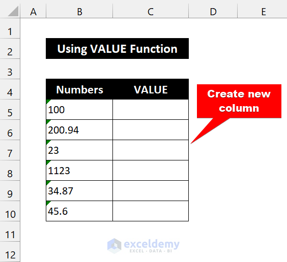
Method 2 – Using the VALUE Function
Steps:
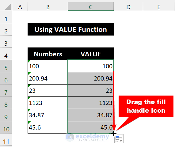
- Create a new column, VALUE, next to the Numbers column.
- Enter the following formula in Cell C5:
=VALUE(B5)
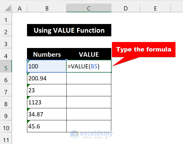
- Press Enter. You will see the text converted to a number.
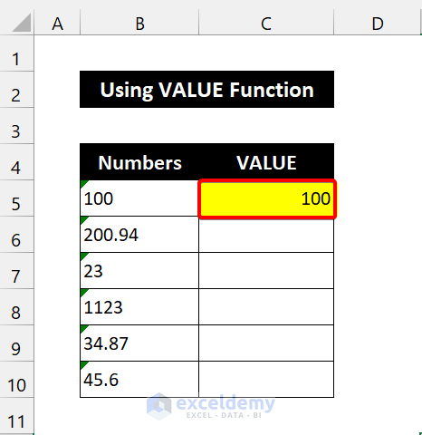
- Drag the fill handle over the cells C6:C10.
Read More: [Solved] Excel Number Stored As Text
Method 3 – Use of the Paste Special Command
Steps:
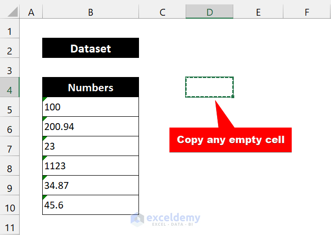
- Copy any empty cell from your worksheet.
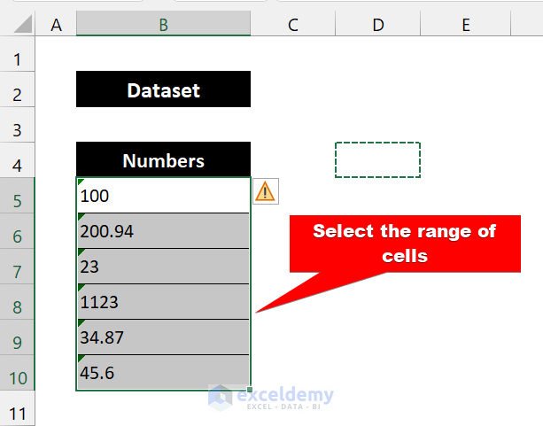
- Select cells B5:B10.
- Rght-click and select Paste Special.
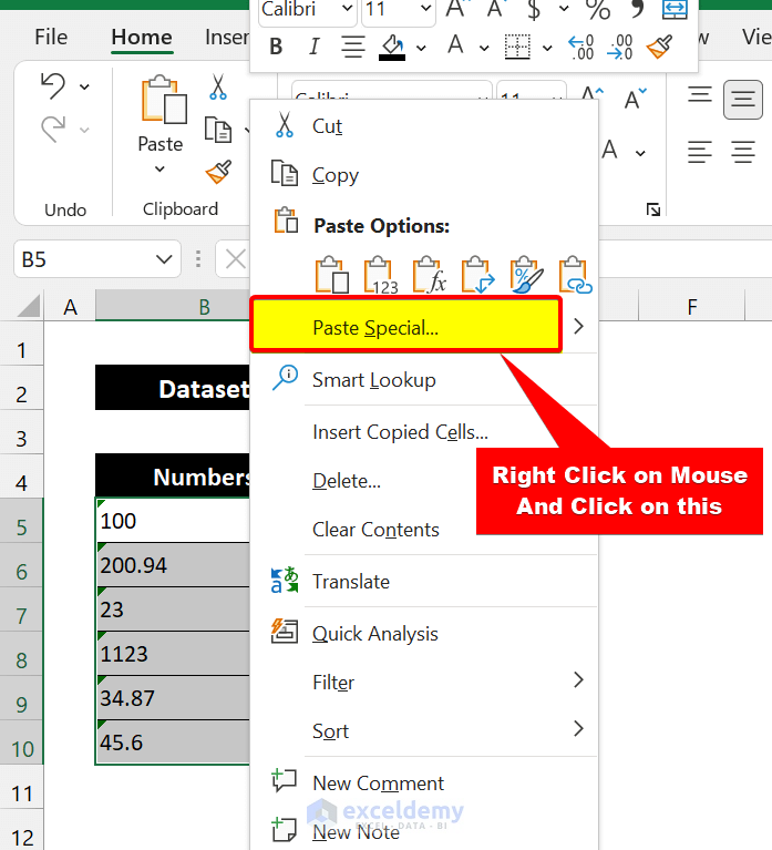
- A Paste Special dialog box will appear. Select the All except borders. Select Add.
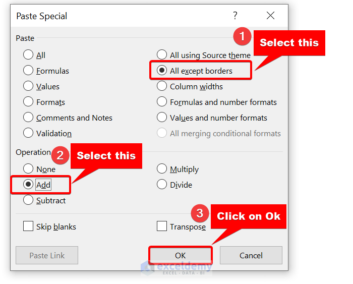
- Click OK.
Read More: How to Custom Format Cells in Excel?
Things to Remember
✎ We are showing the problem in text formats. Your numbers can be in different formats. So, make sure you check the format in the Number group from the Home Tab.
✎ If you use the Number Formats method, it will show a green triangle even after it changes to numbers. You have to double-click the cell to make it right-aligned.
✎ The VALUE function will only work if your numbers are in text form.
Download the Practice Workbook
Download the workbook to practice.
Related Articles
- Apply Engineering Number Format in Excel (2 Easy Ways)
- How to Change International Number Format in Excel (4 Examples)
- Enter 20 Digit Number in Excel (2 Easy Methods)
- How to Enter 16 Digit Number in Excel (3 Simple Ways)
- Display Long Numbers in Excel (4 Easy Ways)


didn’t work for me, I do not have the green triangle in any of my cells; therefore none of your methods worked. I know what the problem is, it is a space after the number finishes, however, I have tried to get rid of the space, but cannot find a way that works via formula, only physically going in to each cell and manually removing the blank space at the end of each number – do you have any solutions for this please?
Hey Luna, you can use VBA codes to solve your problem if these methods don’t work.
Read this article:
https://www.exceldemy.com/convert-text-to-number-excel-vba/
Thank you Shanto, I have tried all the formulas in your link for removing blank space after number; none worked 🙁 The only one I haven’t tried is the VBA code, fingers crossed this one works … I shall let you know. Can I email the spreadsheet to you if not? 🙂
Hey Luna, did you solve the problem using the VBA code? If you face further problems, feel free to share them in the comment box. We are eager to help you to get the desired result.
You should not need VBA, you should be able to use trim() or left() or Right() or mid() functions to remove space. I had a different problem, none of these methods worked for me but on the Home toolbar on the RHS is a Clear Formatting (eraser icon) function. When I did that, and combined it with the =value() function as well as copy and paste values only back into the same column, i was able to fix. Unbeliveable that this is necessary and that Format > Number just does not work sometimes.
Hello JB,
Thank you for your feedback. Admittedly, like everything else, Excel has its downsides too and sometimes the solution to a problem can be quite surprising, but whatever works! Right?
That said, we’re delighted that you’ve shared your experience with us, hopefully, other people find this useful. Have a good day.