This is an overview:
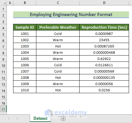
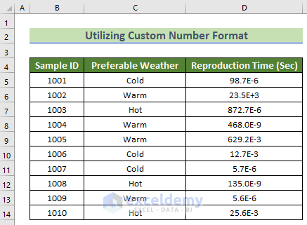
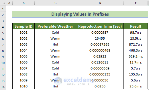
The dataset showcases Sample ID, Preferable Weather, and Reproduction Time (Sec).To show the values of Reproduction Time (Sec) in engineering number format:
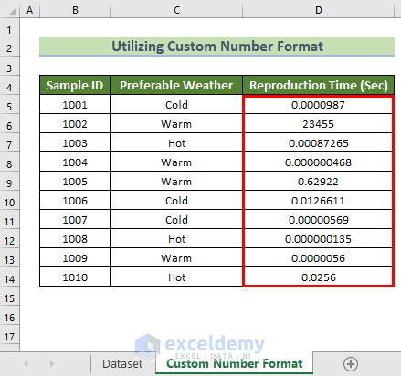
Method 1 – Utilizing Custom Number Format to Apply Engineering Number Format
Steps:
- Select D5:D14.
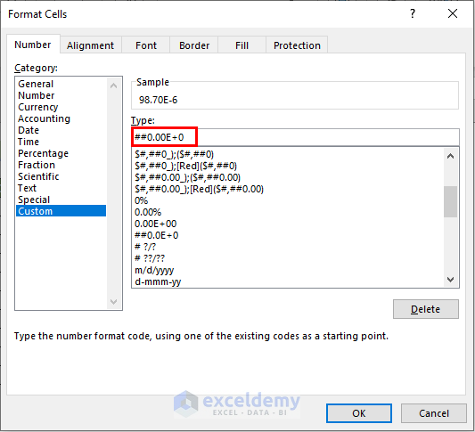
- Press Ctr+1.
- The Format Cells dialog box is displayed.
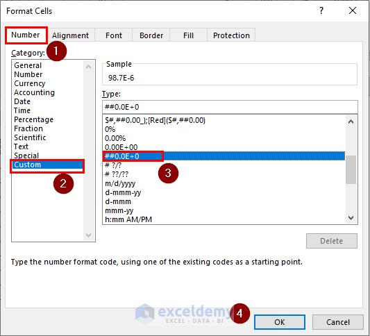
- In Number, select Custom.
- Select ##0.0E+0 in Type:.
- Click OK.
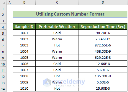
Tips: You can customize the number of decimal places.
Here, more zeros were entered to control decimal places.
This is the output.
Read More: Convert Scientific Notation to Text in Excel
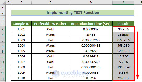
Method 2 -Using the TEXT Function to Get Values in Engineering Number Format
Steps:
- Select E5.
- Enter the following formula:
=TEXT(D5,"##0.0E+0")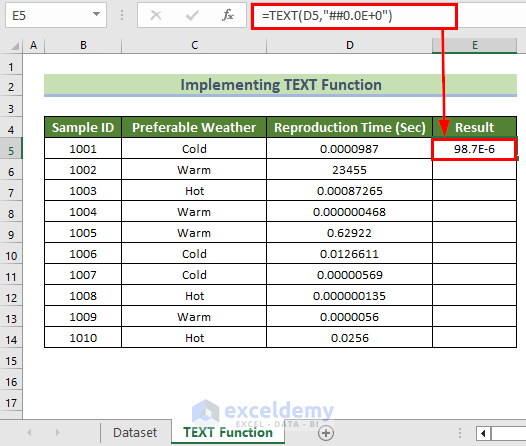
Formula Breakdown
- TEXT(D5,”##0.0E+0″) → The TEXT function converts the value in D5 into engineering format ##0.0E+0.
- Output: 7E-6.
- Drag down the Fill Handle to see the result in the rest of the cells.
Read More: Convert Scientific Notation to Number in Excel
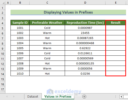
How to Display Values with Units in Engineering Format in Excel?
- Create a Result column to show values in prefixes.
- Select E5.
- Use the following formula:
=LEFT(TEXT(D5,"##0.0E+0"),FIND("E",TEXT(D5,"##0.0E+0"))-1) & MID("npum kMGT",5+VALUE(MID(TEXT(D5,"##0.0E+0"),FIND("E",TEXT(D5,"##0.0E+0"))+1,100))/3,1) &" s"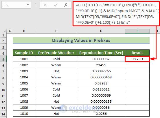
Formula Breakdown
- TEXT(D5,”##0.0E+0″) → The TEXT function converts the value in D5 into engineering format ##0.0E+0.
- Output: 7E-6.
- FIND(“E”,TEXT(D5,”##0.0E+0″)) → becomes
- FIND(“E”, “98.7E-6”) → The FIND function locates E in the string 7E-6 and returns its position.
- Output → 5.
- FIND(“E”, “98.7E-6”) → The FIND function locates E in the string 7E-6 and returns its position.
- LEFT(TEXT(D5,”##0.0E+0″),FIND(“E”,TEXT(D5,”##0.0E+0″))-1) → becomes
- LEFT(“98.7E-6”,4) → The LEFT function returns 4 digits starting from the left of the provided string 7E-6.
- Output → 7.
- LEFT(“98.7E-6”,4) → The LEFT function returns 4 digits starting from the left of the provided string 7E-6.
- MID(TEXT(D5,”##0.0E+0″),FIND(“E”,TEXT(D5,”##0.0E+0″))+1,100) → becomes
- MID(“98.7E-6”,6,100) → The MID function return characters starting from position 6.
- Output → -6.
- MID(“98.7E-6”,6,100) → The MID function return characters starting from position 6.
- VALUE(MID(TEXT(D5,”##0.0E+0″),FIND(“E”,TEXT(D5,”##0.0E+0″)) → becomes
- VALUE(“-6”) → The VALUE function converts the text -6 into a number.
- Output → -6.
- VALUE(“-6”) → The VALUE function converts the text -6 into a number.
- MID(“npum kMGT”,5+VALUE(MID(TEXT(D5,”##0.0E+0″),FIND(“E”,TEXT(D5,”##0.0E+0″))+1,100) → becomes
- MID(“npum kMGT”,3,1) → The MID function returns one character from position 3. (here, n → nano, p → pico, u → micro, m → mili, k → kilo, M → Mega, G → Giga, T → Tera is in npum kMGT)
- Output → u.
- MID(“npum kMGT”,3,1) → The MID function returns one character from position 3. (here, n → nano, p → pico, u → micro, m → mili, k → kilo, M → Mega, G → Giga, T → Tera is in npum kMGT)
- LEFT(TEXT(D5,”##0.0E+0″),FIND(“E”,TEXT(D5,”##0.0E+0″))-1) & MID(“npum kMGT”,5+VALUE(MID(TEXT(D5,”##0.0E+0″),FIND(“E”,TEXT(D5,”##0.0E+0″))+1,100))/3,1) → becomes
- “98.7” &”u” → The & operator returns the combined form of the given values.
- Output → 7u.
- “98.7” &”u” → The & operator returns the combined form of the given values.
- LEFT(TEXT(D5,”##0.0E+0″),FIND(“E”,TEXT(D5,”##0.0E+0″))-1) & MID(“npum kMGT”,5+VALUE(MID(TEXT(D5,”##0.0E+0″),FIND(“E”,TEXT(D5,”##0.0E+0″))+1,100))/3,1) &” s” → becomes
- “98.7u” &” s” → The & operator returns the combined form of the given values.
- Output → 7u s.
- “98.7u” &” s” → The & operator returns the combined form of the given values.
- Drag down the Fill Handle to see the result in the rest of the cells.
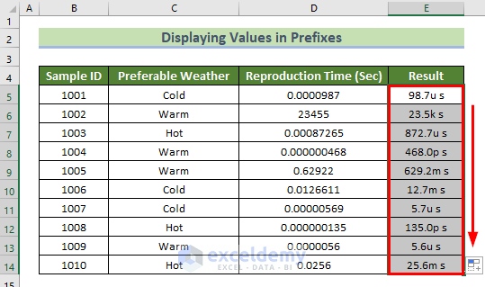
This is the output.
Practice Section
Practice here.

Download Practice Workbook
Download the practice workbook.
Related Articles
- Enter Scientific Notation in Excel
- How to Set Scientific Notation to Powers of 3 in Excel
- How to Remove Scientific Notation in Excel
- Prevent Excel from Converting to Scientific Notation CSV
- Excel Scientific Notation Without e
<< Go Back to Scientific Notation in Excel | Number Format | Learn Excel
Get FREE Advanced Excel Exercises with Solutions!
