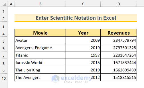
How to Enter Scientific Notation in Excel (4 Methods)

In this article, we’re going to show you 4 methods of how to enter scientific notation in Excel. We’ve taken a dataset containing 3 columns: Movie, Year, and Revenues. We aim to change the formatting of the Revenue column to scientific notation.

1. Using Number Format to Enter Scientific Notation in Excel

We’ll use the Number Format option in Excel to enter scientific notation in this method.

Steps:

Firstly, select the cell range D5:D10.
Secondly, from the Home tab >>> click on the DropDown box from the Number section.

Finally, click on Scientific.

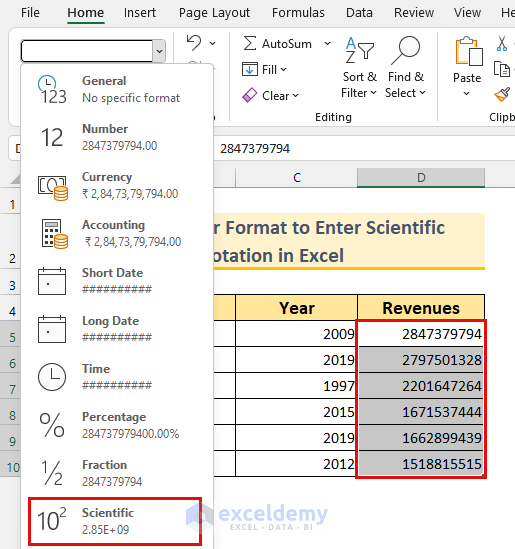
Thus, we’ve entered scientific notation in Excel.

2. Using Excel Format Cells Option to Enter Scientific Notation

For the second method, we’ll use the Format Cells option to enter scientific notation.

Steps:

Firstly, select the cell range D5:D10.
Secondly, right-click to bring up the Context menu.

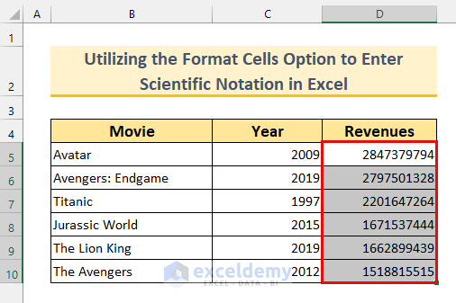
Thirdly, click on Format cells… from the menu.

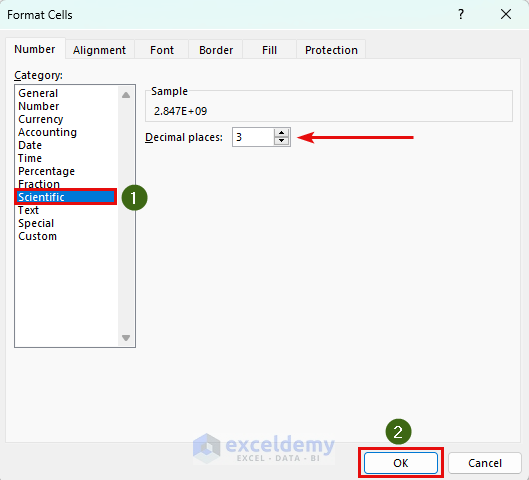
Format Cells dialog box will appear.

Then, from the Category: click on Scientific.
After that, we can change the Decimal places of our number.

Although we’ve set it to 3, this is totally optional.

Finally, click on OK.

In conclusion, we implemented yet another method to enter scientific notation.

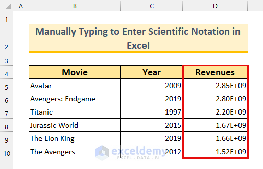
3. Typing Scientific Notation Manually in Excel

We can type in the scientific notation manually too. From the dataset, we can see that there are 10 digits in each Revenue value.

Steps:

Firstly, type “2.847379794e9” in cell D5.

Note: The value “2847379794” from cell D5 can be written as, “2.847379794e9” or “28.47379794e8”. Here, the “e” is not case sensitive, which means “e or E” both will provide the same result.

Secondly, press ENTER.

Here, the value is in scientific notation.

Moreover, we can repeat it for the rest of the cells.

Note: If you have many cells, this method is not efficient for that. Therefore, try the other methods for that.

Read More: How to Display Power in Excel

4. Entering Scientific Notation in Excel and Converting to X10 Format

For the last method, we’ll convert the scientific notation in Excel to X10 format. To do that, we’ll use the LEFT function, the TEXT function, and the RIGHT function.

Steps:

Firstly, type the following formula in cell E5.

=LEFT(TEXT(D5,"0.00E+0"),4) & "x10^" & RIGHT(TEXT(D5,"0.00E+0"),2)

Formula Breakdown

In this formula, we’re using the LEFT and the RIGHT functions to extract the values before and after “E” respectively. On top of that, we’re using the TEXT function to convert the values into the text as in the scientific notation format. Finally, we’re joining the values with the ampersands.

TEXT(D5,”0.00E+0″)
- Output: “2.85E+9”.
- The TEXT function converts the value into text in the scientific notation.
LEFT(“2.85E+9”,4)
- Output: “2.85”.
- The LEFT function returns the values up to the 4th position from the left side.
RIGHT(“2.85E+9”,2)
- Output: “+9”.
- The LEFT function returns the values up to the 2nd position from the right side.
Finally, our formula reduces to, “2.85” & “x10^” & “+9”
- Output: “2.85×10^+9”.
- We’re joining the values with the ampersands.

Secondly, press ENTER.

Thus, we’ve changed our format.

Finally, AutoFill the formula using the Fill Handle.

In conclusion, we’ve changed the scientific notation to the “X10” format.

Download Practice Workbook

Enter Scientific Notation.xlsx

Conclusion

We’ve shown you 4 methods of how to enter scientific notation in Excel. Moreover, if you face any problems understanding these, feel free to comment below. Thanks for reading; keep excelling!