In Excel, we can easily calculate the value of different power/exponent of different base values. But they are often not shown in the traditional power/exponential format that we are used to seeing in doc files. They show the value of those exponents directly on the cell. But for presentation purposes, users sometimes need to demonstrate the real source or reason behind that data. For this, we need to show the exponentials of different variables in Excel. To help on this issue, 5 separate easy and time-saving methods discuss by which you will be able to display power in Excel efficiently.
Display Power in Excel: 6 Simple Ways
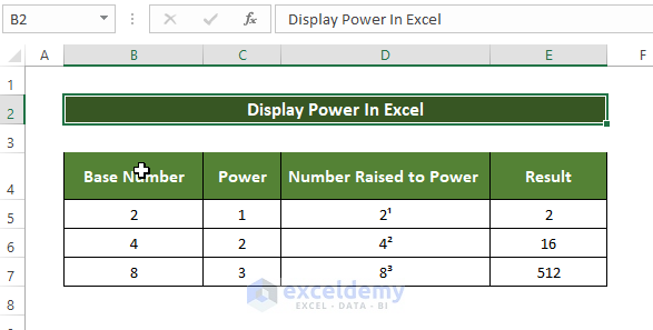
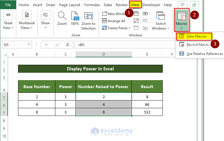
To demonstrate how to format the phone number with dashes, we are going to use the following spreadsheet random numbers in the Base Number column and which power they are going to be raised is shown in the Power column. The result or the display of the power using the various methods will be shown in Number Raised to Power. And the numerical result of those raising power is shown in the Result Column.
Read More: How to Enter Scientific Notation in Excel
1. Show Power in Excel with Formula
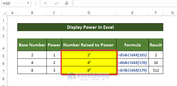
This method is restricted to only 1-3. That means numbers can only be raised from 1 to 3. In this process, you can preserve the original number. You just have to concatenate the original number with the CHAR function given below,
For raising power to 1, use code =CHAR(185).
To raise the power to 2, use code =CHAR(178).
For raising power to 3, use code =CHAR(179).
📌 Steps
- Select the Cell D5, enter the following Formula:
=B5&CHAR(185)
- After that, press Enter.
- After that, the value in Cell B5 will raises to power 1.
- Similarly, repeat the process for Cell D6, enter the following formula:
=B6&CHAR(178)
- Then, press Enter.
- After that, the value in Cell B6 will raises to power 1.
- After that repeat the same process for Cell D7, enter the following formula:
=B7&CHAR(179)
- Then, press Enter.
- After that, the value in Cell B7 will raises to power 1.
- All of these formulas are mentioned from Cell E5 to Cell E7.
After following this procedure, you will see that all the values in Cell B5 to Cell B7 are raised to the power mentioned in Cell C5 to Cell C7 correspondingly.
Read More: How to Set Scientific Notation to Powers of 3 in Excel
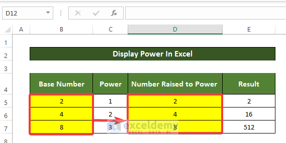
2. Display Power in Excel Utilizing Custom Formatting
In this process, the numbers are transformed into a Custom format.
📌 Steps
- First, copy the cells from column B5:B7 to column D5:D7 like the following.
- Then select Cell D5, and right-click on it. From the context menu select Format Cell.
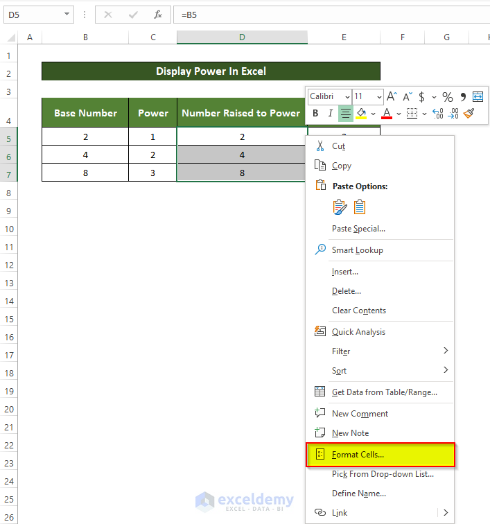
- After clicking the Format Cell option, go to Number > Custom > Type And type 0.

- Then the most important part, here, in the Type field, after entering 0, hold Alt, enter 0185, then release Alt.
- After releasing Alt, you will notice that the power of 0 is now showing 1. This means our Custom formatting is successful. Click OK after that.

- After clicking OK, you will notice that the number in Cell D5 now has the power of 1.
- Similarly, if you repeat this for other Cells with corresponding Character Codes, they will also have power as shown below.

Read More: How to Convert Scientific Notation to Text in Excel
3. Keyboard Shortcut to Display Power in Excel
In this method, you are going to raise numbers to power using simple Excel shortcuts.
📌 Steps
- First, copy the cells range of cells B5:B7 to D5:D7.

- We need to use the shortcut key mentioned in the column named Shortcut from Cell D5 to Cell D7.
- Next, select Cell E5, double-click to enter edit mode, hold Alt, then type 0185. After that, release Alt.

- After releasing Alt, the power of 2 in Cell E5 is going to 1.

- Similarly, repeat the same procedure through Cell E5 to Cell E7, and apply the appropriate shortcut keys mentioned in the Shortcut column, then all the mentioned numbers will display their raised power.

Note:
1. This method works only for Calibri and Ariel fonts. For other fonts, Character Codes might be different. So it is better to avoid it if you are using other fonts.
2. After performing the shortcuts, these cell values are converted into Numeric strings, which means you can’t perform calculations with them.
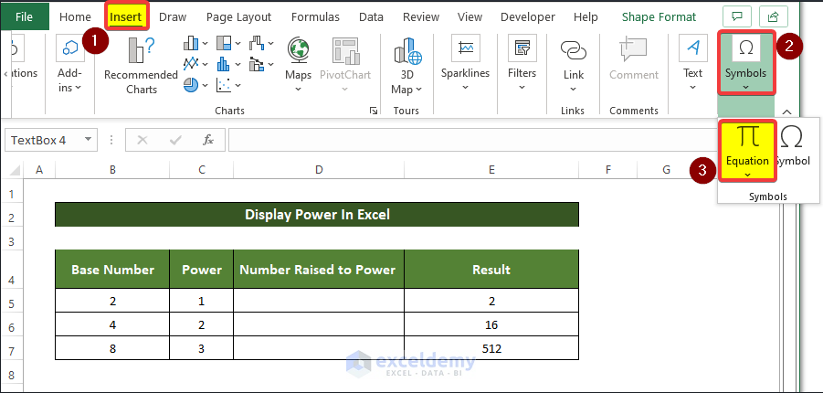
4. Display Power Using Equation Option in Excel
In this method, we are going to use the equation option from the Symbols command.
📌 Steps
- First, go to the Insert tab. After that click on Symbols > Equation.
- After clicking Equation, go to Structures > Script.
- Then choose the first box, from the Subscripts and Superscripts, the one shows the left box one lower and the right box is higher,
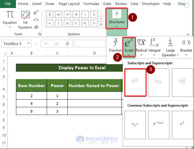
- A new box will appear, in that box, type the base Number and the power.
- Then move the box to Cell D6.
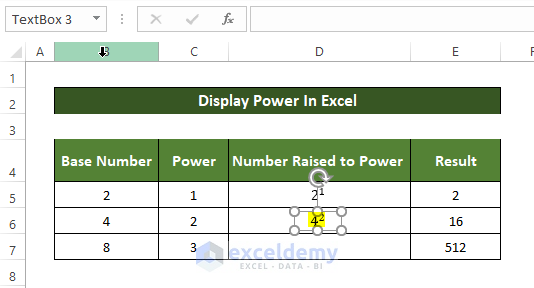
- Repeat the same for other numbers. Then you will have a complete list of numbers raised to the corresponding power.
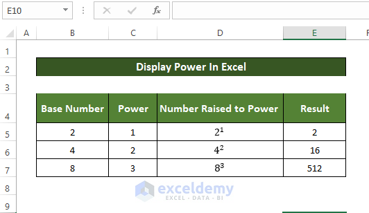
Note: This method enters the value raised in power just as an Excel object, not a Cell input actually. So basically you can just display the value, but can’t use that value for referencing actually. so for the referencing and calculation work, avoid this method.
5. Superscript Format Command in Format Cell Option
In this process, the Superscript Function can be used to display the power of the numbers.
📌 Steps
- Firstly, you have to write the power of the Number listed in the Power column in Cell C5 through Cell C7 right next to the Base Numbers.

- Next in the Number raised to Power Column, double click Cell D5 and carefully select only the Power Section(which was from the Power column, Cell C5).
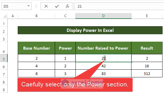
- After selecting the Power Section only, right-click on the mouse, and from the context menu, select the Format Cells option. You can also open the Format Cells option by pressing F2 to enter edit mode, and then pressing Ctrl+1.

- A new dialog box will open, from that, check the box in the Superscript.

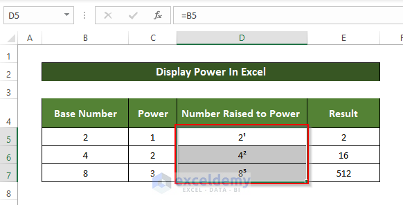
- Next, click the Number in Cell D5 will raise it to power 1.

- Like other methods, if you repeat the process for other numbers, You will display the power of the numbers.
6. Using VBA Macro to Display Power in Excel
A simple code in the VBA macro can easily solve the task. Utilizing macros is quite hassle-free and time-saving.
📌 Steps
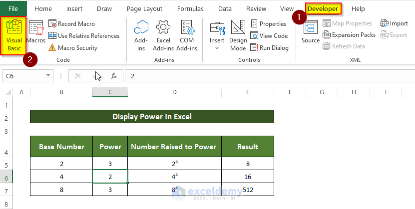
- Launch the Visual Basic Editor from the Developer tab.
- Pressing Alt + F11 on your keyboard can also launch the Visual Basic editor.
- After launching the Visual Basic editor, a new window will launch.
- In the new window click Insert, then click Module.
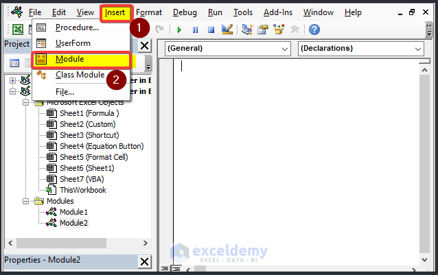
- Next, a white editor will open. In that editor, you need to write the following code:
Sub display_power()
    Selection.NumberFormat = "0" & Chr(179)
End Sub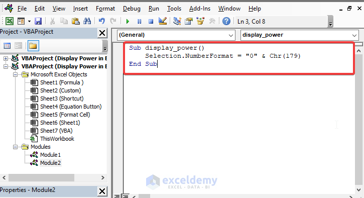
- Upon writing the code, close both the Module and the VBA editor.
- Select the numbers you wish to raise power, then from the View tab, click the Macros command, then select the View Macros option.
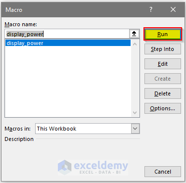
- Next, a new dialog box will open, from that dialog box, select the macro display power that you just created and click Run.
- Upon clicking Run, you will notice that all the numbers display and raised to power.
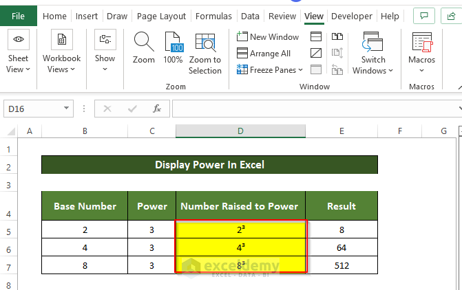
You can use these numbers for other references and calculations.
Download Practice Workbook
Download this practice workbook from the button below.
Conclusion
To sum it up, the question “how we can display power in Excel“ can be answered in six principal ways. Among those methods, method 1 to 3 is restricted to only power 1 to 3. That means you can’t raise numbers above 3. But methods no 4 and 5 are quite flexible and allow users to raise their number to whatever power they need to raise. And at last, the power of the numbers raises utilizing a VBA macro. This method is the most time-saving and simplest one.
A workbook containing a dataset with all the methods done is available for download for practice. Feel free to ask any questions or feedback through the comment section.
Related Articles
- Remove Scientific Notation in Excel
- Convert Scientific Notation to Number in Excel
- Prevent Excel from Converting to Scientific Notation CSV
- Excel Engineering Number Format
- Excel Scientific Notation Without e
<< Go Back to Scientific Notation in Excel | Number Format | Learn Excel
Get FREE Advanced Excel Exercises with Solutions!
