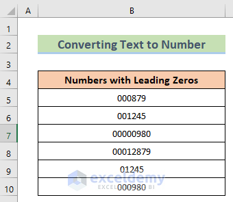
Method 1 – Converting Text to Number to Remove Leading Zeros in Excel
Steps:
- Arrange a dataset like the below image.
- Select the Convert to Number option from the error mark.
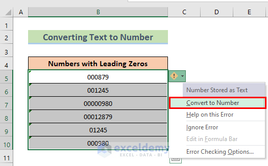
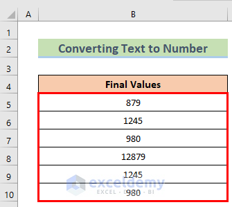
- You will get the desired result.
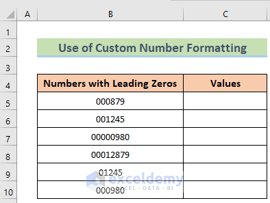
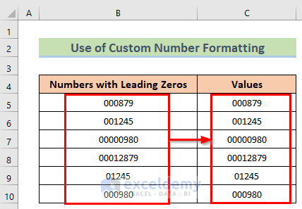
Method 2 – Using the Custom Number Format in Excel to Remove Leading Zeros
Steps:
- Arrange a dataset like the below image.
- Copy the full Column B using the Ctrl+C buttons and paste it to Column D using the Ctrl+V option.
- Go to select the desired column > Home > General options.
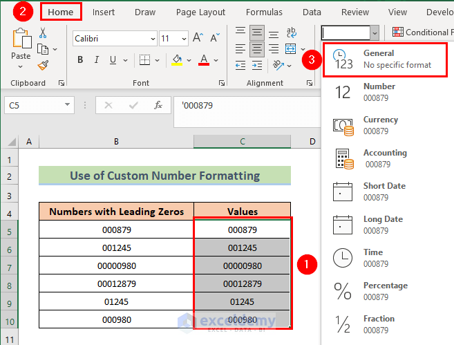
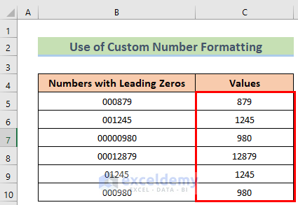
- You will get the desired result.
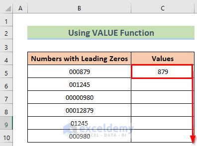
Method 3 – Inserting the VALUE Function to Remove Leading Zeros
Steps:
- Arrange a dataset like the below image, and in the C5 cell insert the following formula.
=VALUE(B5)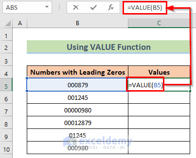
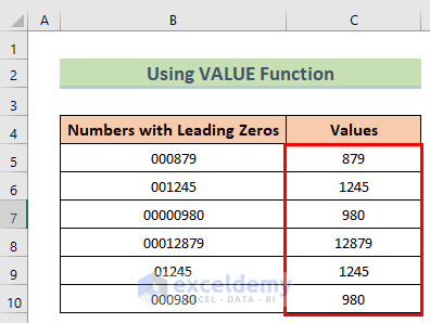
- If you press the Enter button, you will get the result for the cell and then use the Fill Handle to apply the formula to all the desired cells.
- Get the desired result.
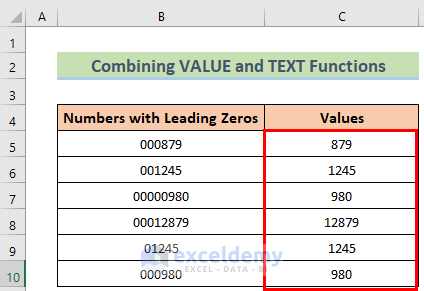
Method 4 – Combining VALUE and TEXT Functions to Remove Leading Zeros
Steps:
- Arrange a dataset like the below image, and in the C5 cell insert the following formula.
=TEXT(VALUE(B5), "#")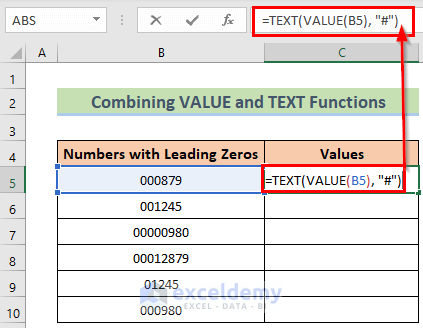
- Press the Enter button, you will get the result for the cell and then use the Fill Handle to apply the formula to all the desired cells.
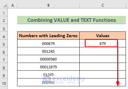
- Get the desired result.
How Does the Formula Work?
- VALUE(B5): This portion represents the cell you want to convert.
- TEXT(VALUE(B5), “#”): This portion represents the whole condition according to our wish.
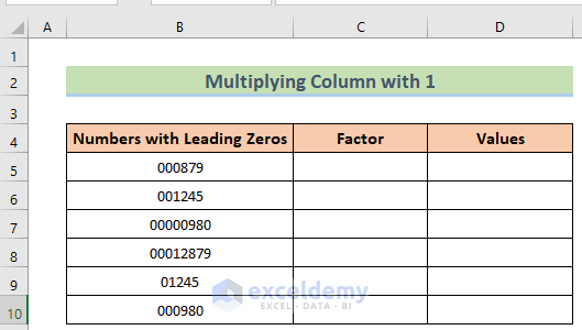
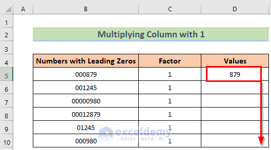
Method 5 – Removing Leading Zeros by Multiplying a Column with 1
Steps:
- Arrange a dataset like the below image.
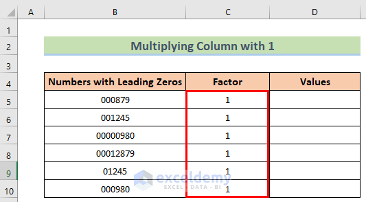
- Insert 1 in all the cells of Column C.
- In the D5 cell, insert the following formula.
=B5*C5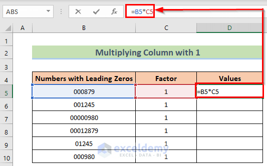
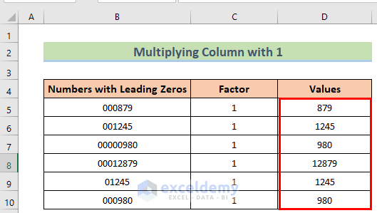
- Press the Enter button, you will get the result for the cell and use the Fill Handle to apply the formula to all the desired cells.
- Get the desired result.
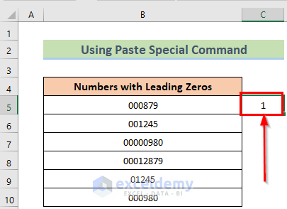
Method 6 – Using the Excel Paste Special Command to Remove Leading Zeros
Steps:
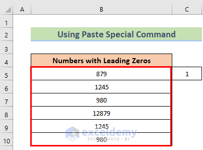
- Arrange a dataset like the below image, and in the C5 cell, insert 1 and copy it using Ctrl + C buttons.
- Right-click on the desired column and select the Paste Special option.
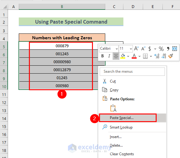
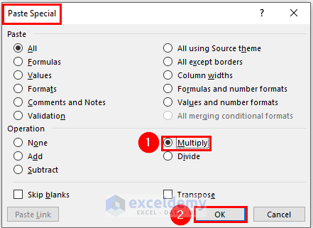
- The Paste Special dialog box will open.
- Select the Multiply option and click OK.
- You will get the desired result.
Method 7 – Removing Leading Zeros with the Text to Columns Feature
Steps:
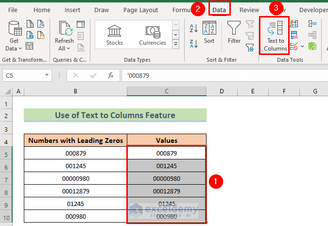
- Arrange a dataset like the below image and go to select the desired cell.
- Go to Data and then to Text to Columns.
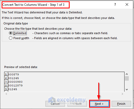
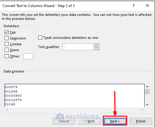
- In the 1st dialog box, press the Next option.
- In the 2nd dialog box, press the Next option.
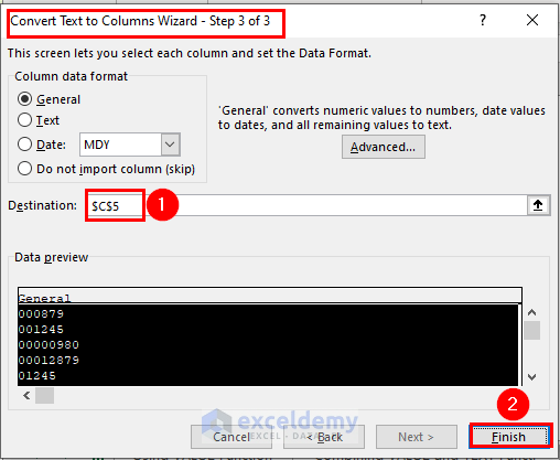
- Select the desired column in the destination for the 3rd dialog box section and press the Next option.
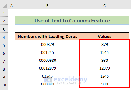
- Get the desired result.
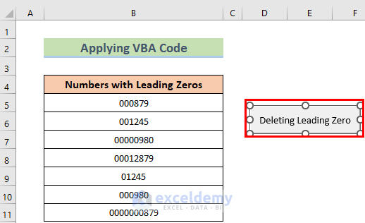
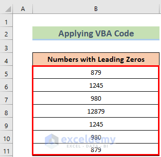
Method 8 – Applying Excel VBA Tool for Removing Leading Zeros
Steps:
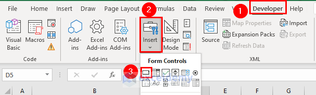
- Go to Developer > Insert > Form Controls.
- Draw a button with your mouse (click and drag, then release).
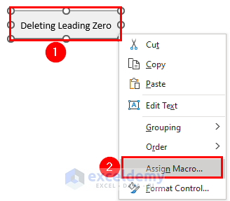
- Right-click on the button and select the Assign Macro option.
- Insert the VBA code here.
Sub Removing_Leading_Zero()
'Code by ExcelDemy.com
Dim Remove_Range As Range
Dim Wrk_Rng As Range
On Error Resume Next
xTitleId = "ExcelDemy Delete Leading Zeros"
Set Wrk_Rng = Application.Selection
Set Wrk_Rng = Application.InputBox("Range", xTitleId, Wrk_Rng.Address, Type:=8)
Wrk_Rng.NumberFormat = "General"
Wrk_Rng.Value = Wrk_Rng.Value
End Sub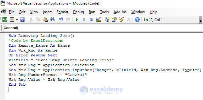
- Select the desired data range and press the button option.
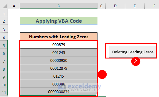
- Get the desired result.
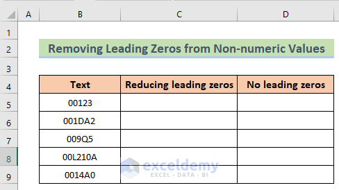
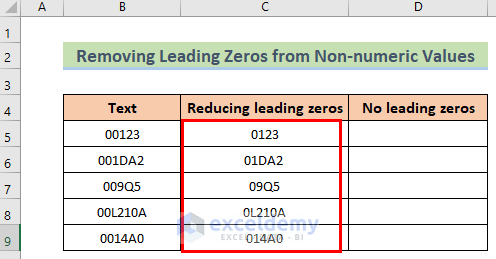
How to Remove Leading Zeros from Non-Numeric Values in Excel
Steps:
- Arrange a dataset like the below image.
- In the C5 cell insert the following formula.
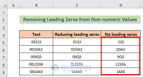
=IF(LEFT(B5) = "0", RIGHT(B5, LEN(B5)-1), B5)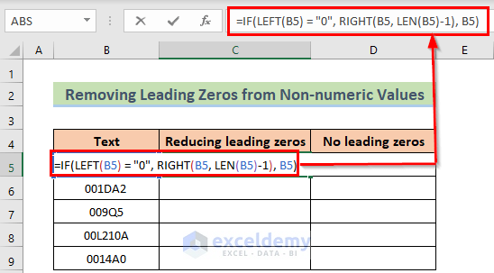
- If you press the Enter button, you will get the result for the cell and then use the Fill Handle to apply the formula to all the desired cells.
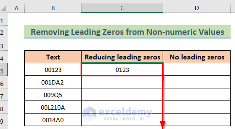
- Get the result for this column.
- Apply the steps for Column D, then you will get the desired result.
Download the Practice Workbook
Related Articles
- How to Keep Leading Zero in Excel Date Format
- How to Add Trailing Zeros in Excel
- How to Keep Leading Zeros in Excel CSV
<< Go Back to Pad Zeros in Excel | Number Format | Learn Excel
Get FREE Advanced Excel Exercises with Solutions!

Very good, congratulations
FERREIRA, Thanks for your feedback!
Hi Kawser, Thanks for the lessons
Hello Johmono,
You’re most welcome.
Thanks for your feedback.
Best regards