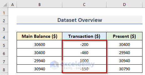
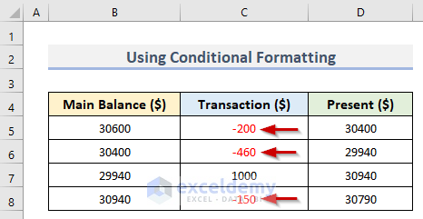
Let’s use a dataset (B4:D8) in Excel that contains the Main Balance, Transaction and Present Balance. We can see 3 negative numbers in cells C5, C6, and C8 respectively. Now, we will make these negative numbers red by using some features in Excel.
Method 1 – Using Conditional Formatting to Make Negative Numbers Red in Excel
Steps:
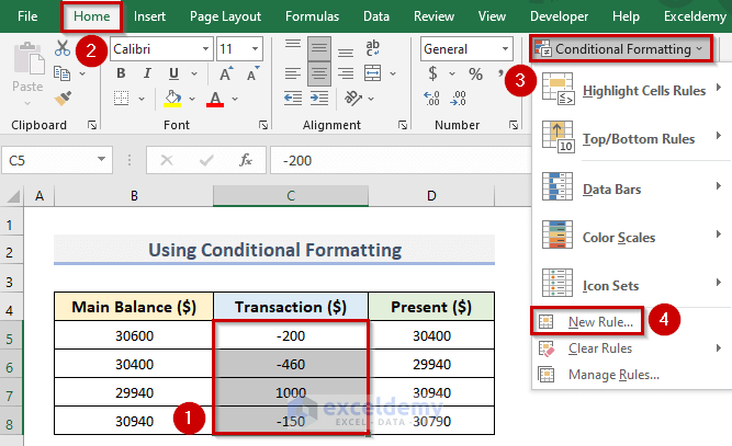
- Select the range (C5:C8) where you want to apply Conditional Formatting.
- Go to the Home tab.
- Click on the Conditional Formatting dropdown in the Styles group.
- Select New Rule from the dropdown.
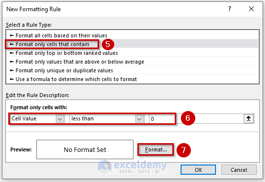
- The New Formatting Rule dialog box will pop up.
- Click on ‘Format only cells that contain’ from the Select a Rule Type section.
- Go to the Format only cells with section and select Cell Value and less than for the first two sections from the dropdown.
- In the third section, type 0.
- Click on Format to choose the font color.
- The Format Cells dialog box will appear.
- Go to the Font tab and choose a Red color from the dropdown.
- Click OK.
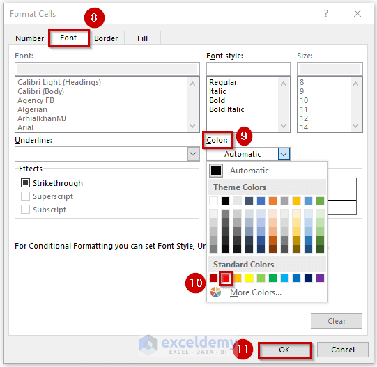
- You should see the red font color in the Preview section.
- Click OK to apply the formatting in the selected range (C5:C8).

- Here are the negative numbers in cells C5, C6 and C8 in a red color.
Read More: How to Add Brackets to Negative Numbers in Excel
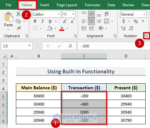
Method 2 – Showing Negative Numbers in Red with Built-In Excel Functionality
Steps:
- Select the specific range (C5:C8) where you have the negative numbers.
- Go to the Home tab.
- Go to the Number group and click on the Number Format dialog launcher.
- Choose the Dialog launcher at the bottom right of the group.
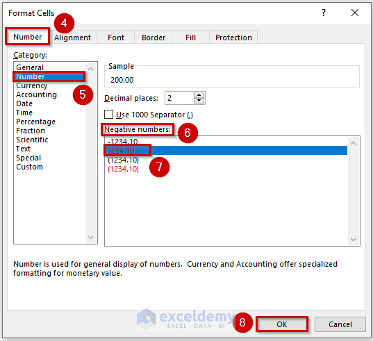
- The Format Cells dialog box will show up.
- Go to the Number tab.
- Select Number from the Category section.
- Go to the Negative numbers section.
- Select the number with red color.
- Click OK.
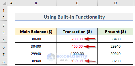
- This makes the negative numbers red.
Read More: Excel Negative Numbers in Brackets and Red
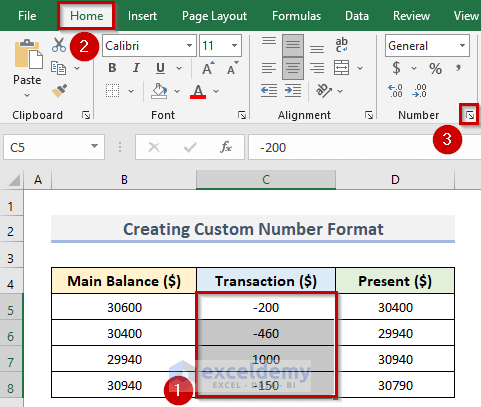
Method 3 – Creating a Custom Number Format to Mark Negative Numbers in Red
Steps:
- Select the desired range (C5:C8).
- Go to the Home tab and click on the Number Format dialog launcher.
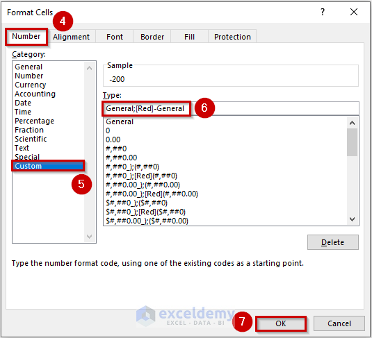
- You’ll see the Format Cells dialog box.
- Go to the Number tab.
- Select Custom in the Category section.
- Select the Type box on the right.
- Insert the following line in the box: General;[Red]-General
- Click the OK button.
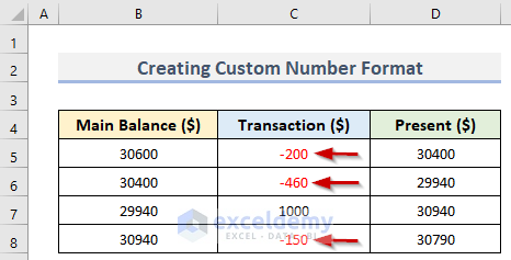
- All the negative numbers of the selection are expressed in red.
Read More: How to Put Negative Percentage Inside Brackets in Excel
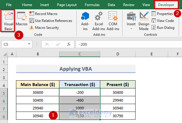
Method 4 – Applying Excel VBA to Make Negative Numbers Red
Steps:
- Select the range C5:C8.
- Go to the Developer tab.
- Click on Visual Basic.
- The Microsoft Visual Basic for Applications window will open up.
- Click on Insert and select Module.
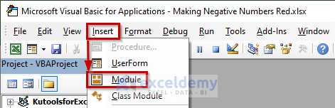
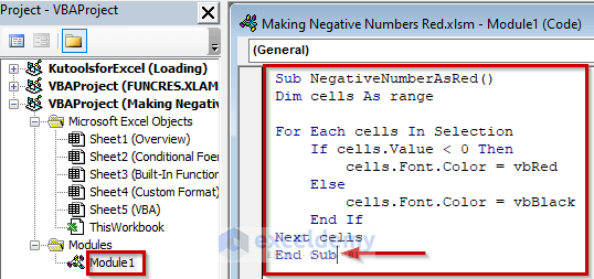
- The Module1 window will appear.
- Insert the following code in the window:
Sub NegativeNumberAsRed()
Dim cells As range
For Each cells In Selection
If cells.Value < 0 Then
cells.Font.Color = vbRed
Else
cells.Font.Color = vbBlack
End If
Next cells
End Sub- You must keep the cursor in the last line of the code (see the screenshot below) before running the code.
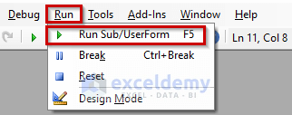
- Click on Run and select Run Sub/UserForm.
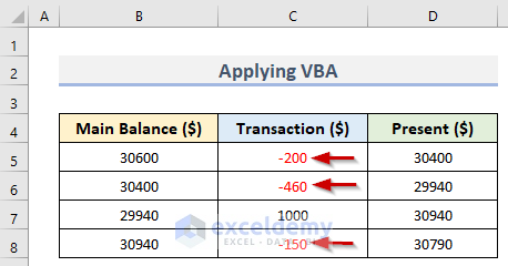
- We will see the negative numbers in red.
Download the Practice Workbook
Related Articles
- Excel Formula for Working with Positive and Negative Numbers
- How to Move Negative Sign at End to Left of a Number in Excel
- How to Put Parentheses for Negative Numbers in Excel
- How to Sum Negative and Positive Numbers in Excel
- How to Change Positive Numbers to Negative in Excel
<< Go Back to Negative Numbers in Excel | Number Format | Learn Excel
Get FREE Advanced Excel Exercises with Solutions!
