How to Add Brackets to Negative Numbers in Excel (3 Easy Ways)

Get FREE Advanced Excel Exercises with Solutions!

It is a common case while working in Excel to get negative values in the calculation. By default, Excel will put a negative sign before such values. But if you want to emphasize these values for research or experimental purposes, then you can add brackets to these negative numbers for better visualization. In this article, we will show you how to add brackets to negative numbers in Excel.

Table of Contents hide

Download Practice Workbook

3 Easy Ways to Add Brackets to Negative Numbers in Excel

1. Changing Cell Format to Add Brackets to Negative Numbers in Excel

2. Customizing Format Cells Box to Add Brackets to Negative Numbers in Excel

3. Applying VBA to Add Brackets to Negative Numbers

Conclusion

Download Practice Workbook

You can download the free Excel workbook here and practice on your own.

Add Brackets to Negative Numbers.xlsm

3 Easy Ways to Add Brackets to Negative Numbers in Excel

While you are using Excel for accounting purposes or calculating the profit or loss of an enterprise or institution, it is very common to get negative values as a result. To emphasize these values for a better analysis, you may want to visualize them properly. Adding brackets to those numbers can be a great way of visualizing. In this article, you will find three different ways to add brackets to negative numbers in Excel. We will change the cell format of these numbers in our first method, customize the Format Cells box in the second one, and apply a VBA code in our last approach. 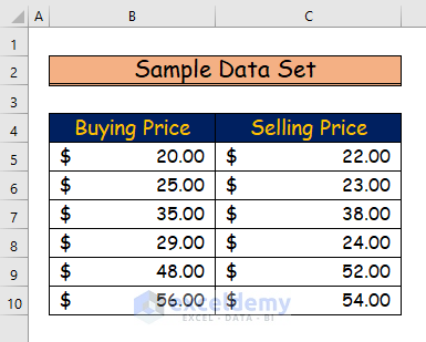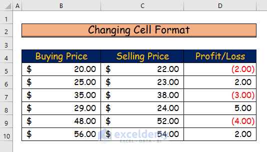For our working purposes, we will use the following data set. Here we have the buying price and selling price of some products.

1. Changing Cell Format to Add Brackets to Negative Numbers in Excel

You can change the cell format of the desired cell value and then add brackets to those negative numbers. For the detailed procedure, see the following steps.

Step 1:

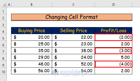
First of all, we will calculate the expected profit or loss from our data set.
To do this, type the following formula into cell D5.

=B5-C5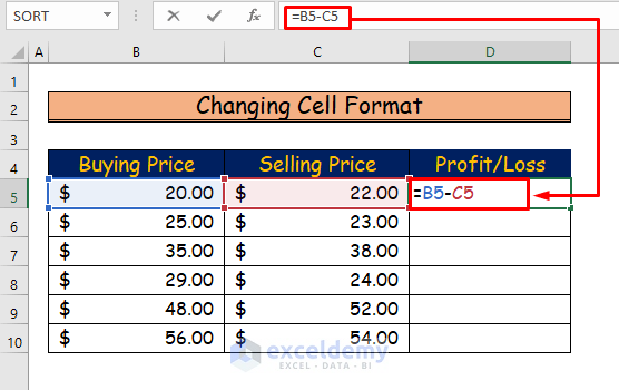

Step 2:

Secondly, press Enter to see the result.
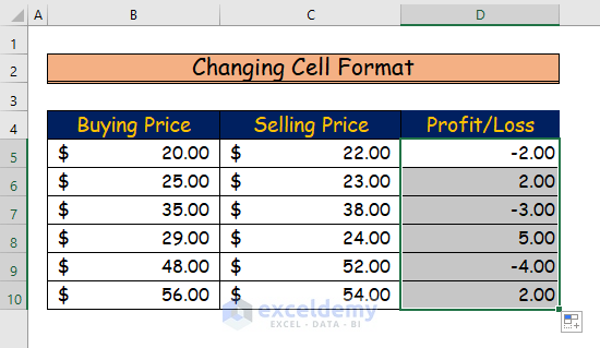
Then, use the AutoFill feature to drag the formula for the lower cells of the same column.

Step 3:

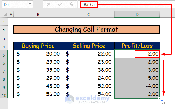
Thirdly, you will notice negative numbers in the data set after calculation.
Hence, we will add brackets to these numbers.
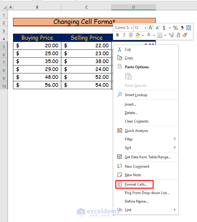
To do this, first of all, select all the numbers from cell range D5:D10.

Step 4:

Fourthly, right-click on the mouse after selecting the cell range.
Then, select the Format Cells… command.

Step 5:

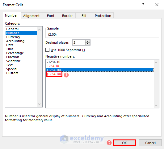
Fifthly, you will see the Format Cells dialogue box.
Then, go to the Number tab of the box.
From there, choose the Number option.

Step 6:

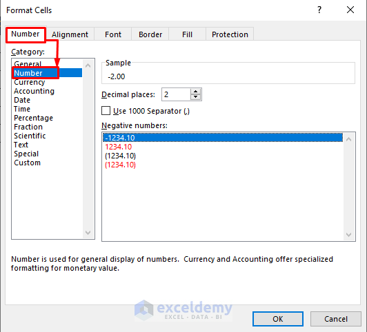
In the sixth step, from the option, choose the command (1234.10), which is in black.
Then, press OK.

Step 7:

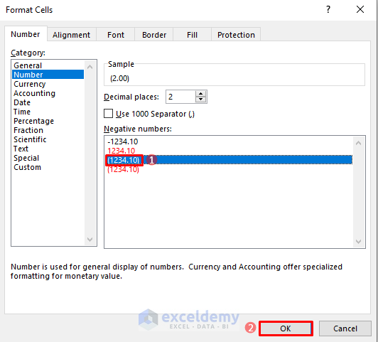
After that, you will see all the negative numbers in column D are in brackets and in black.

Step 8:

Furthermore, if you want to change the color of the negative numbers with brackets, then go to the Number options from the Format Cells dialogue box.
Then, choose the command (1234.10) which is in red.
Lastly, press OK.

Step 9:

Finally, you will see all the negative numbers in brackets and their color will be red.

2. Customizing Format Cells Box to Add Brackets to Negative Numbers in Excel

You can also customize the Format Cells box to add brackets to negative numbers. The steps are as follows.

Step 1:

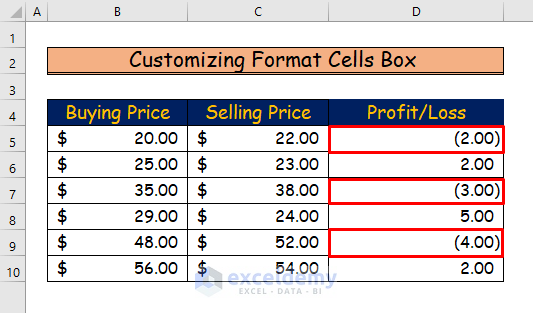
First of all, select the cell range where you want to add brackets.
For our example, the cell range is D5:D10.
Then, go to the Home tab of the ribbon.
From there, in the Number group, choose the little arrow on the lower-right side of the group.

Step 2:

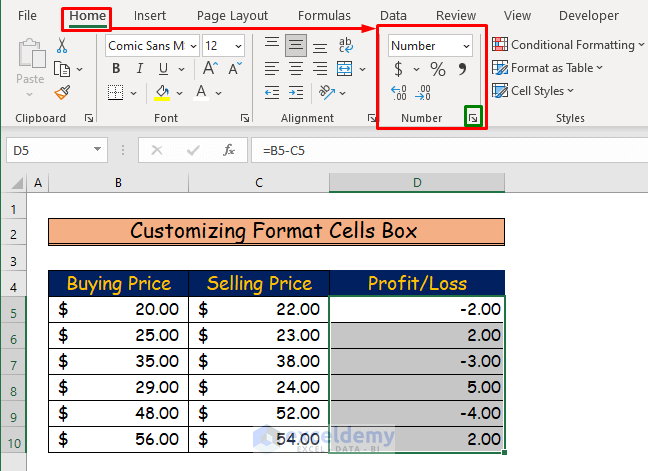
Secondly, you will see the Format Cells dialogue box.
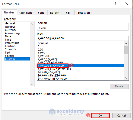
Then, go to the Custom tab from the box.

Step 3:

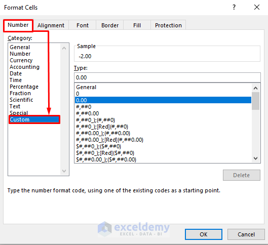
Thirdly, from the tab, choose the command #,##0.00_);(#,##0.00).
Then press OK.

Step 4:

Fourthly, this command will add brackets to the negative numbers in the data set.
Consequently, they will be black in color.

Step 5:

Fifthly, if you want your bracketed negative numbers in red color then choose the #,##0.00_);[Red](#,##0.00) command from the Format Cells dialogue box.

Then, press OK.

Step 6:

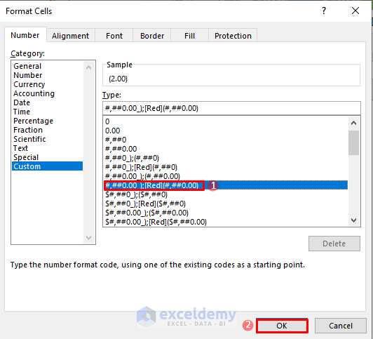
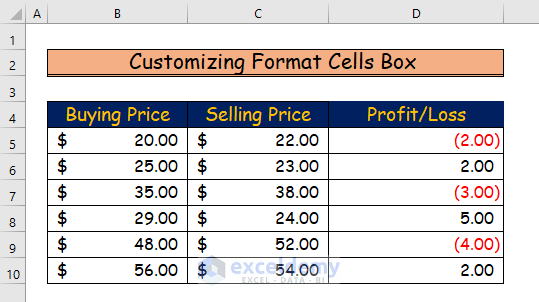
Finally, this command will show all the negative numbers in red with brackets.

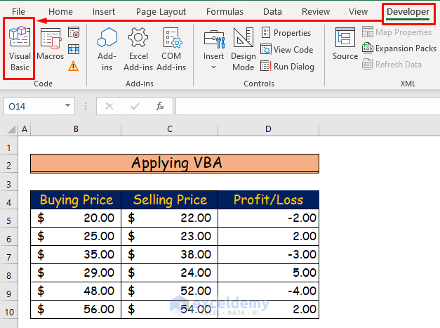
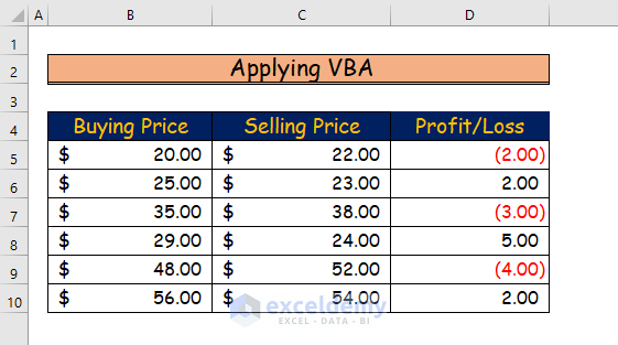
3. Applying VBA to Add Brackets to Negative Numbers

Lastly, we will apply a VBA code to our data set to accomplish the task. The following steps will give you a complete guideline.

Step 1:

Firstly, go to the Developer tab of the ribbon.
Then, choose the Visual Basic command from the Code group of the tab.

Step 2:

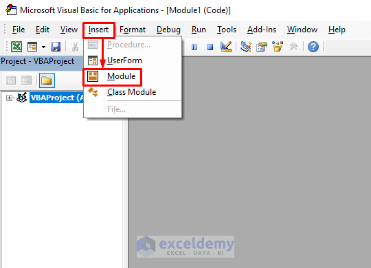
Secondly, you will see the VBA window after selecting the command.
Then, from the Insert tab choose Module.

Step 3:

Thirdly, paste the following VBA code in the module.

'Set the Function Name
Sub Add_Brackets_to_Negative_Numbers()
'Select the Cell range where the negative numbers are
Range("D5:D10").Select
'Set the format of the cells after adding brackets
Selection.NumberFormat = "0.00_);[Red](0.00)"
End Sub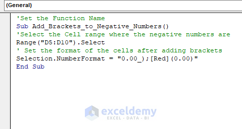

VBA Breakdown

The function name is Add_Brackets_to_Negative_Numbers.
Range(“D5:D10”).Select: Select the cell range where the negative numbers are located.
Selection.NumberFormat = “0.00_);[Red](0.00)”: Add brackets to negative numbers and set their font color as red.

Step 4:

Fourthly, save the code and then press the play button or F5 to run the code.

Step 5:

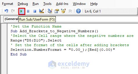
Finally, you will see all the negative numbers in brackets after running the code.

Conclusion

That’s the end of this article. I hope you find this article helpful. After reading the above description, you will be able to add brackets to negative numbers in Excel by using any of the above-described methods. Please share any further queries or recommendations with us in the comments section below. The Exceldemy team is always concerned about your preferences.