How to Show Negative Numbers in Brackets and in Red in Excel (2 Methods)

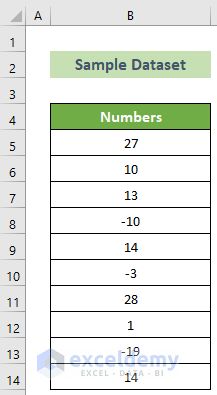
Dataset Overview

We will use a dataset containing 10 numbers of which 3 are negative.

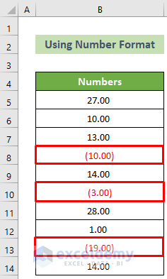
Method 1 – Using Excel’s Format Cells Option 

The easiest and quickest way to show Excel negative numbers in brackets and red is to customize the Number format.

Follow the steps below to do this.

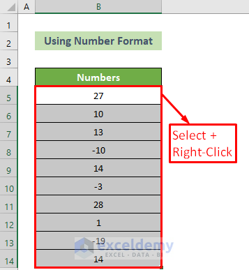
• Select all the cells in the dataset.
• Right-click on your mouse button.

• Choose the Format Cells… option from the Context Menu.

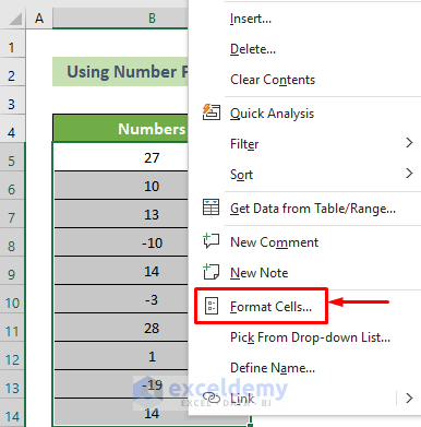
• The Format Cells dialogue box will appear.
• Go to the Number tab >> choose Number from the Category pane >> choose the last option (1234.10) from the Negative numbers pane >> click OK.

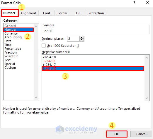
You will see all the negative numbers of your dataset in brackets and red color.

Read More: How to Change Positive Numbers to Negative in Excel

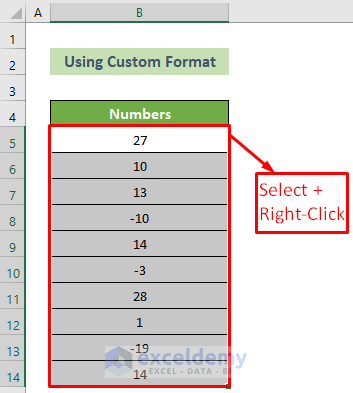
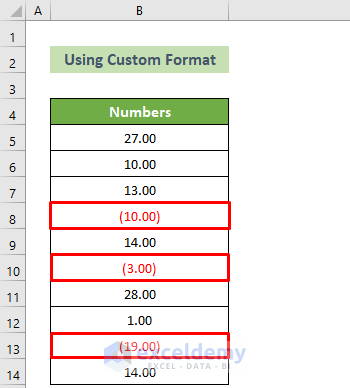
Method 2 – Applying a Custom Format 

Another effective way to show negative numbers in brackets and red is to use the Custom Format.

Follow the steps below to do this.

• Select the dataset and right-click on your mouse.

• Choose the Format Cells… option from the Context Menu.

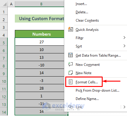
• The Format Cells dialogue box will appear.
• Go to the Number tab >> Custom option from the Category pane >> insert the following format in the Type text box:

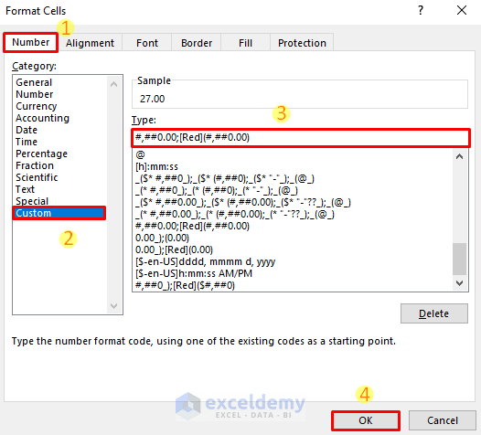
• Click OK.

You will get all the negative numbers displayed in brackets and red color.

Read More: How to Make Negative Numbers Red in Excel 

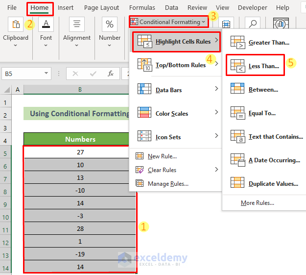
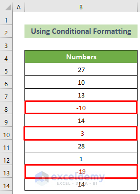
How to Show Excel Negative Numbers in Red Color with Conditional Formatting

You can also use conditional formatting to display negative numbers in red color but without brackets.

• Select the dataset.
• Go to the Home tab >> Conditional Formatting tool >> Highlight Cells Rules option >> Less Than… option.

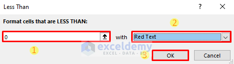
• The Less Than dialogue box will appear.
• Enter the value 0 in the Format cells that are LESS THAN text box.
• Choose the Red text option from the with options.
• Click OK.

All the negative numbers in the dataset will be red in color.

Read More: How to Add Brackets to Negative Numbers in Excel

Download Practice Workbook

You can download the practice workbook from here:

Related Articles

• How to Put Negative Percentage Inside Brackets in Excel
• How to Put Parentheses for Negative Numbers in Excel
• How to Move Negative Sign at End to Left of a Number in Excel
• Excel Formula for Working with Positive and Negative Numbers
• How to Sum Negative and Positive Numbers in Excel

<< Go Back to Negative Numbers in Excel | Number Format | Learn Excel