We often have negative numbers in our Excel dataset. Negative numbers can create a problem while calculating in Excel. So, it is important to count the negative numbers present in a dataset. In this article, we will discuss how to count negative numbers in Excel.
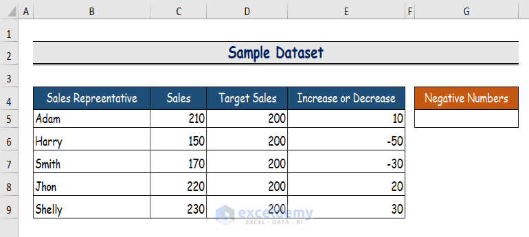
In this blog, we will discuss 3 effective methods to count negative numbers in Excel. In the first method, we will use the COUNTIF function to count the negative numbers. Next, we will opt for the SUMPRODUCT function to do the task. Finally, we will use a VBA code to do our calculation. We will use the following sample dataset to carry out our method illustrations.
1. Using COUNTIF Function to Count Negative Numbers in Excel
In this method, we will use the COUNTIF function to count the negative numbers. Follow the subsequent steps to carry out the task.
Step 1:
- Firstly, choose the cell in which to display the outcome of the count of the negative numbers.
- In this instance, the cell is G5.
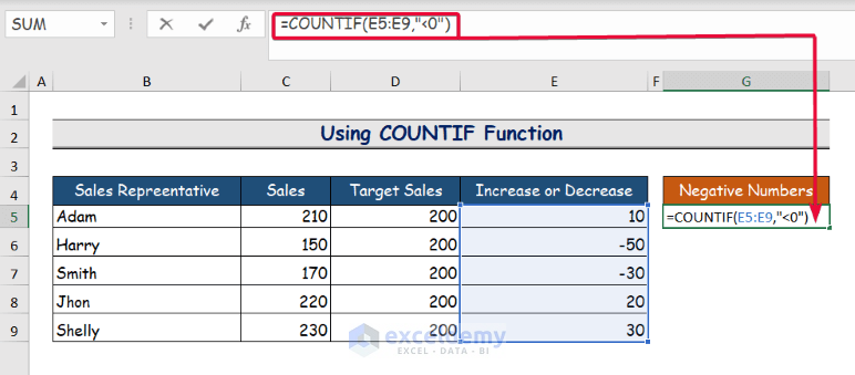
- Then, write the following formula in cell G5.
=COUNTIF(E5:E10,"<0")- Here, E5:E10 is the range of cells where you want to search for the negative numbers.
- “<0” or “less than zero” is the condition on which the function will return the result.
- This function returns an array of True and False.
- To convert those True and False into numbers 0 and 1, we will use the two negative signs at the beginning of the function.
- Finally, hit Enter.
Step 2:
- As a result, the cell will display the quantity of negative numbers in the chosen cell range.
- In our case, the result is 2.

Read More: How to Add Negative Numbers in Excel
2. Applying SUMPRODUCT Function to Count Negative Numbers
In this example, we will opt for the SUMPRODUCT function to count the negative numbers. Follow the ensuing steps to do it.
Step 1:
- Firstly, decide which cell will contain the results of the count of the negative numbers.
- In this instance, we will select the G5 cell.
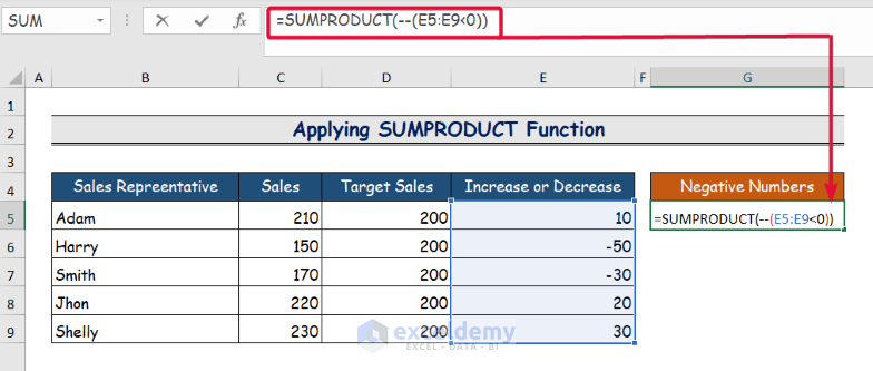
- After that, enter the following formula into cell G5.
=SUMPRODUCT(--(E5:E10<0))- In this case, the range of cells where you want to look for the negative numbers is E5:E10.
- The condition on which the function will return the result is “0” or “less than zero“.
- Lastly, press Enter.
Step 2:
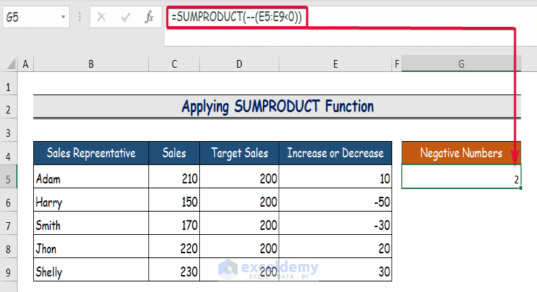
- Consequently, the cell will return the number of negative numbers in the selected range of cells.
- In our case, the result is 2.
Read More: How to Show Negative Numbers in Excel
3. Use of Excel VBA Code to Count Negative Numbers
In this method, we will resort to a VBA code to count the numbers of the negative numbers in our dataset. Adhere to the outlined steps below to complete the task.
Step 1:
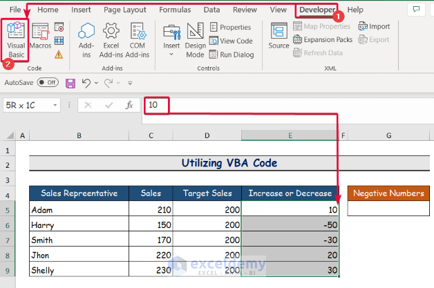
- Firstly, select the range of cells where you want to look for the negative numbers.
- In our case, the range is E5:E10.

Step 2:
- Secondly, go to the Developer tab.
- From the Developer tab, select the Visual Basic command.
- Consequently, a Visual Basic dialogue box will appear.
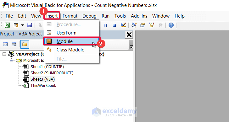
Step 3:
- Thirdly, in the Visual Basic tab, click on Insert.
- Then, select the Module option.
- Consequently, a coding Module will appear.
Step 4:
- In the coding module, write down the following code.
- Then, save the code.
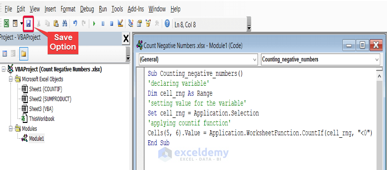
Sub Counting_negative_numbers()
'declaring variable'
Dim cell_rng As Range
'setting value for the variable'
Set cell_rng = Application.Selection
'applying the COUNTIF function'
Cells(5,6).Value = Application.WorksheetFunction.CountIf(cell_rng, "<0")
End Sub
VBA Code Breakdown
- Dim cell_rng As Range: Here, we will declare the variable as Range type variable.
- Set cell_rng = Application.Selection: This implies that the cell_range variable will be assigned the value of the selected range of cells.
- Cells(5,6).Value = Application.WorksheetFunction.CountIf(cell_rng, “<0”): This means, the COUNTIF function will go through the values of the cell_rng variable which is in this case the values in the selected range of cells. The function will impose its condition which is all values that are less than zero in all the cells and return the number of values which satisfies the condition.
Step 5:
- Finally, go to the Run tab and click on it.
- From the drop-down option, select the Run command to run the code.

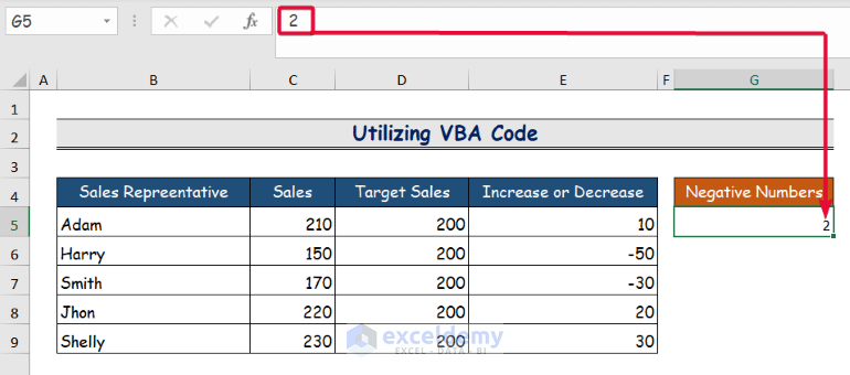
Step 6:
- As a result, you will find that Excel will return the number of negative numbers from the selected range.
- In this instance, the result is 2.
Read More: How to Put a Negative Number in Excel Formula
Download the Practice Workbook
Conclusion
Negative numbers in a dataset could be a tricky business. So, Excel users need to keep track of the negative numbers. The users can easily do that by counting the negative numbers. After going through this article, the readers will have three effective methods to count the negative numbers in their dataset. Please feel free to leave a comment if you have any queries or recommendations for improving the article’s quality. Happy Learning!
Related Articles
- [Fixed!] Excel Not Adding Negative Numbers Correctly
- How to Make a Group of Cells Negative in Excel
- Excel Formula to Return Zero If Negative Value is Found
- Excel Formula If Cell Contains Negative Number
- Excel Formula to Return Blank If Cell Value Is Negative
<< Go Back to Negative Numbers in Excel | Number Format | Learn Excel
Get FREE Advanced Excel Exercises with Solutions!
