In this article, we will show how to convert negative value to positive in Excel using formula. We will create Excel formulas with common functions like IF, MAX, and ABS. Using these formulas, you can easily convert the format. So, without any delay, let’s start the discussion.
How to Convert Negative Value to Positive Using Formula in Excel: 3 Easy Ways
To demonstrate the methods, we will use a dataset of the company’s income for the previous month and the present month in million dollars. By subtraction process, we can find the change in income. Sometimes, we need to know only the value of the difference, not the sign. Let’s see the 3 methods to convert the negative value to the positive using formula in Excel.

1. Use ABS Function to Convert Negative Value to Positive in Excel
Utilizing the ABS function, we can formulate a formula to convert the negative value to positive. Let’s follow the steps below to learn the method.
STEPS:
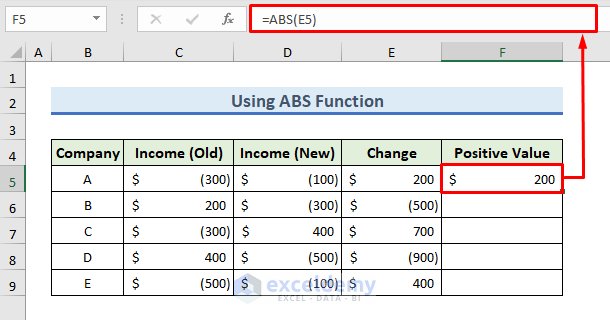
- In the Change column, you can observe both positive and negative numbers.
- In this step, we will convert the negative values of the E column into positive ones.
- To do so, write down the following formula in the F5 cell:
=ABS(E5)- Now, press Enter to see the result.
- After that, drag down the formula in the F6:F9 range with the Fill Handle option.

- As a result, in the Positive Value column, all values are positive.
- So, we have successfully converted the negative value to positive.

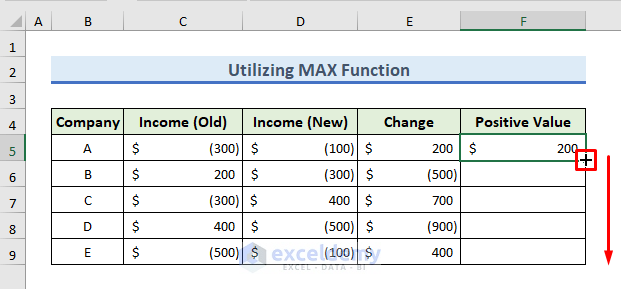
2. Utilize MAX Function to Convert Negative Value to Positive in Excel
Utilizing the MAX function, we can build up a formula to convert the negative value to a positive. Let’s follow the steps below to learn the method.
STEPS:
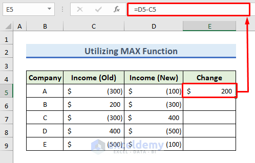
- Firstly, we need to calculate the change in the income of the company.
- To do so, you have the subtraction from the present value to the previous value.
- So, write down the following formula in the E5 cell to calculate the change:
=D5-C5- Then, press OK to observe the result.
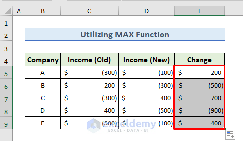
- After that, drag down the subtraction formula in the E6:E9 range with the Fill Handle option.

- As a result, we can observe the change in income in the E column.
- In the Change column, you can observe both positive and negative numbers.
- In this step, we will convert the negative value into positive.
- To do so, write down the following formula in the F5 cell:
=MAX(E5,-E5)- Then, press Enter to watch the result.

- After that, drag down the formula in the F6:F9 range with the Fill Handle option.
- As a result, in the Positive Value column, all values are positive.
- So, we have successfully converted the negative value to positive one.

3. Create a Formula Using IF Function to Change Negative Value to Positive
Utilizing the IF function, we can form a formula to convert the negative value to positive. Let’s follow the steps below to learn the method.
STEPS:
- In the Change column, you can observe both positive and negative numbers.
- In this step, we will convert the negative values of the E column into positive.
- To do so, write down the following formula in the F5 cell:
=IF(E5>0,E5,-E5)- Now, press Enter to see the result.
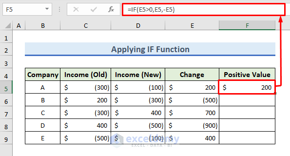
- After that, drag down the formula in the F6:F9 range with the Fill Handle option.

- As a result, in the Positive Value column, all values are positive.
- So, we have successfully converted negative value to positive.

Read More: How to Change Positive Numbers to Negative in Excel
How to Change Negative Value to Positive and Vice Versa in Excel Applying VBA Code
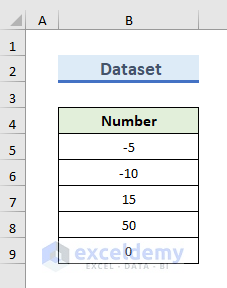
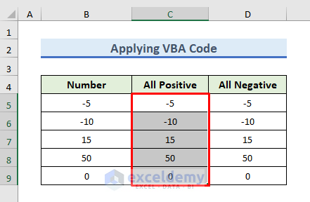
Without building the formula, we can also change the negative value to positive applying VBA Code. Here, you can also change the positive number to negative. To demonstrate the method we have created a dataset of 5 random numbers. Here, both positive and negative numbers are present.
STEPS:
- Firstly, select the numbers in the B4:B9 range.
- Then, Ctrl + C to copy the numbers.
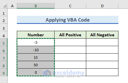
- After that, Ctrl + V to paste the numbers in the C and D columns.
- So, the numbers of the B columns are copied to the C and D columns.

- Now, select the C5: C9 range.
- After selection, click on the Developer tab and select Visual Basic.

- Instantly, the Microsoft Visual Basic Application window will open.
- In this window, select Insert >> Module to open the module.
- In the module, you will insert your code.

- As a result, the module will appear.
- Now, write down the following code in the module:
Sub Pos_To_Neg()
Dim x As Range
For Each x In Selection
If IsNumeric(x.Value) Then
x.Value = Abs(x.Value)
End If
Next x
End Sub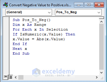
- After writing the code, you need to run the code.
- To do so, press on the following icon.
- So, your code has successfully run.
- Now, return the Excel Worksheet to observe the outcome.

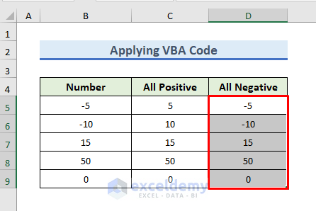
- As a result, in the All Positive column, all values are positive.
- So, we have successfully converted the negative value to positive.

- In the next step, we will convert the positive value to negative.
- To do so, select the D5:D9 range and return to the module.
- In the module, replace the following code with the previous code:
Sub Neg_To_Pos()
Dim x As Range
For Each x In Selection
If IsNumeric(x.Value) Then
x.Value = -Abs(x.Value)
End If
Next x
End Sub- After writing the code, press the following icon to run the code.
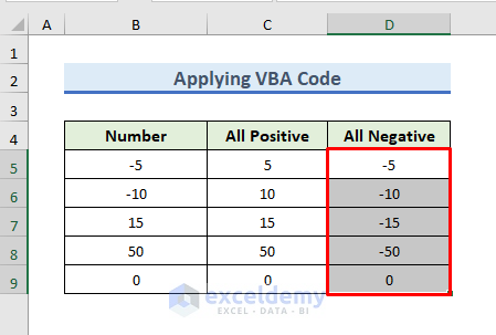
- Now, return the Excel Worksheet to observe the outcome.

- As a result, in the All Negative column, all values are negative.
- So, we have successfully converted the positive value to negative.
Read More: How to Move Negative Sign at End to Left of a Number in Excel
Utilize Custom Formatting to Show Negative Value to Positive and Vice Versa
Utilizing Custom Formatting, we can easily change the negative value to positive and vice versa. Let’s follow the steps below to learn the method.
STEPS:
- Firstly, select the numbers in the B4:B9 range.
- Then, Ctrl + C to copy the numbers.
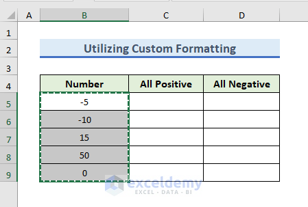
- After that, Ctrl + V to paste the numbers in the C and D columns.
- So, the numbers of the B columns are copied to the C and D columns.

- Now, select the C5: C9 range.

- After selection, press the shortcut key Ctrl + 1.
- Here, the shortcut key will open the custom formatting options.
- Now, go to the Custom panel and in the Type input bar, enter “#,###;#,###”.
- In the end, click OK to proceed.
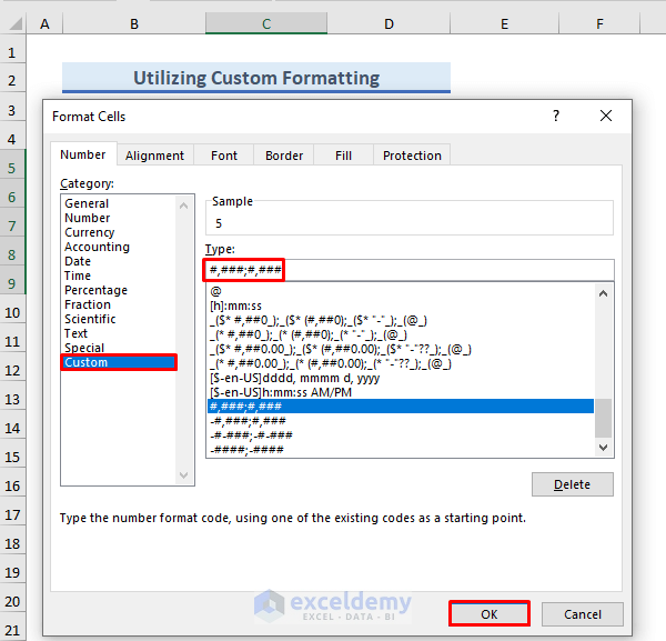
- As a result, in the C column, all the numbers are in the positive form.
- As the C9 cell contains 0, it is showing nothing in this cell.
- After that, you can also convert the positive value to negative.
- So, select the D5: D9 range.

- After selection, press the shortcut key Ctrl + 1.
- Here, the shortcut key will open the custom formatting options.
- Now, go to the Custom panel and in the Type input bar, enter “-#,###;-#,###”.
- In the end, click OK to proceed.
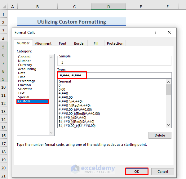
- As a result, in the D column, all the numbers are in the negative form.
- As the D9 cell contains 0, it is showing just (–) in this cell.

Read More: How to Sum Negative and Positive Numbers in Excel
Download Practice Workbook
To practice by yourself, download the following workbook.
Conclusion
In this article, we have shown how to convert negative value to positive in Excel using formula. There is a practice workbook at the beginning of the article. Go ahead and give it a try. Last but not least, please use the comment section below to post any questions or make any suggestions you might have.
Related Articles
- How to Put Negative Percentage Inside Brackets in Excel
- How to Put Parentheses for Negative Numbers in Excel
- How to Add Brackets to Negative Numbers in Excel
- How to Make Negative Numbers Red in Excel
- Excel Negative Numbers in Brackets and Red
- Excel Formula for Working with Positive and Negative Numbers
<< Go Back to Negative Numbers in Excel | Number Format | Learn Excel
Get FREE Advanced Excel Exercises with Solutions!
